
Airborne Tipper Inversion#
This section focuses on the inversion of airborne tipper data generated from the Flin Flon resistivity model.
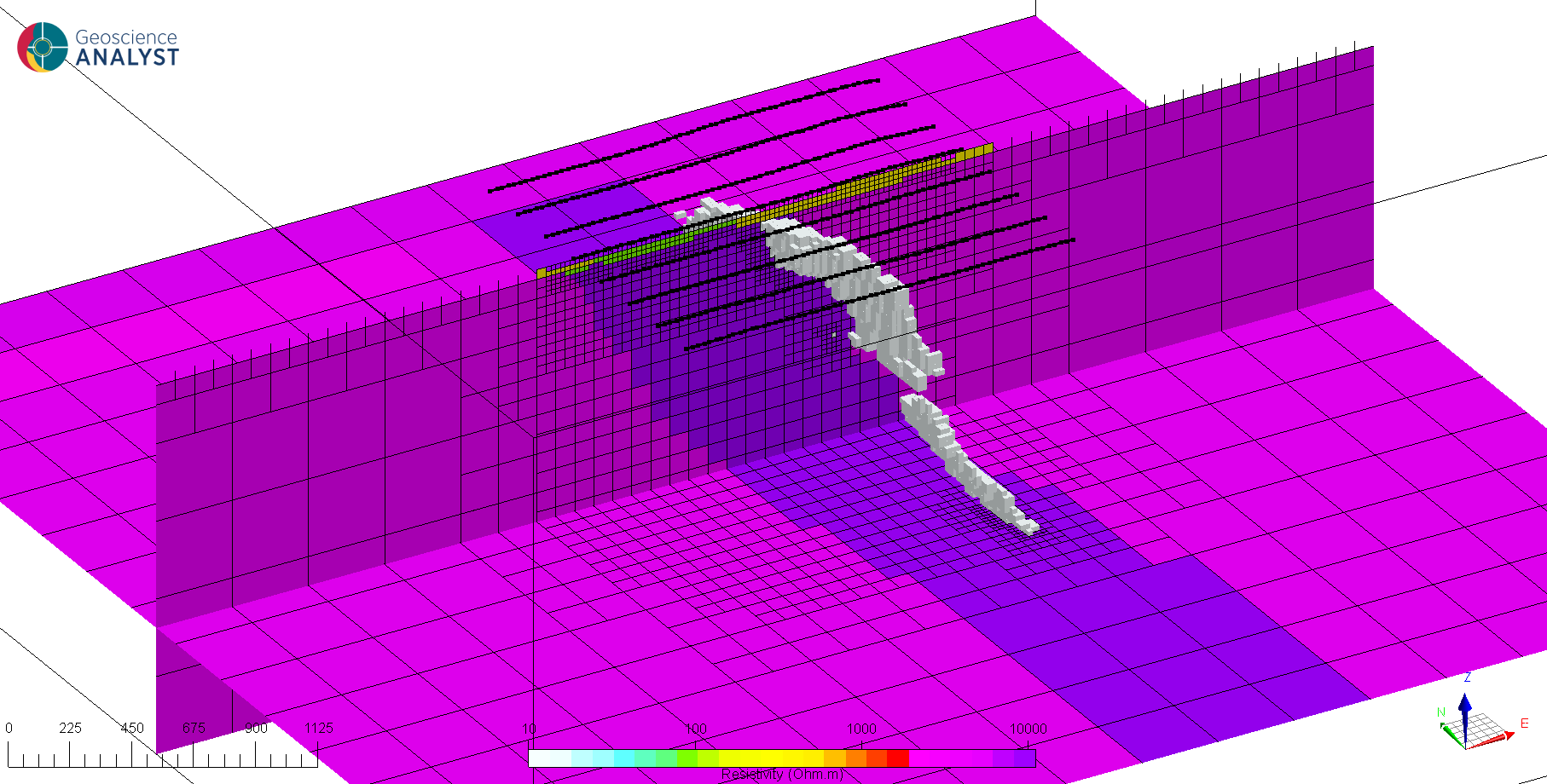
Fig. 28 Download here#
Note
Runtime and memory usage increases rapidly with the mesh size and number of sources (frequencies). It is strongly recommended to downsize this example to a few lines if the training is done on a standard computer. The full inversion presented below was performed on an Azure HC44rs node (44 CPUs, 315 Gb RAM) in ~2.0 h.
Airborne tipper (Natural Source EM)#
We generated an airborne tipper survey over the main ore body. The survey lines are spaced at 400 m, oriented East-West, at a drape height of 60 m.
Tipper systems collect three orthogonal components of the ambient magnetic field (\(H_x,\;H_y,\;H_z\)). Similar to magnetotelluric surveys, the ratios of the components are used to circumvent the unknown source of the EM signal. The transfer functions, or tipper, are calculated by taking the ratio of the fields for two polarizations of the magnetic fields (EW and NS). The measurements are generally provided in the frequency-domain with both a real and an imaginary component. For more background information about natural source methods, see em.geosci
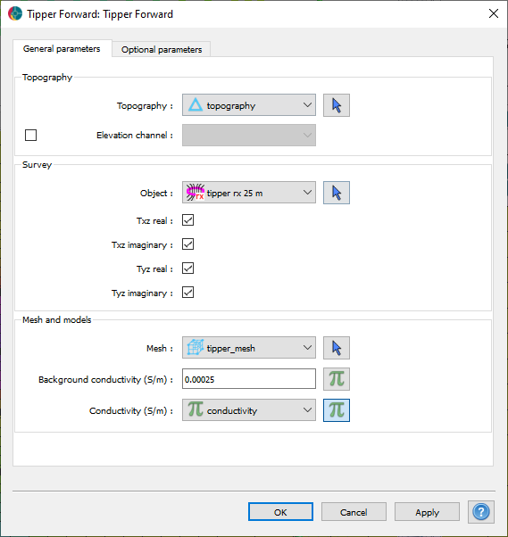
The survey used here mimics the commercial ZTEM system that measures the vertical magnetic field (\(H_z\)) on a towed platform at 6 frequencies (30, 45, 90, 180, 360 and 720 Hz). The horizontal fields (\(H_{x,y}\)) are measured at a fixed base station located in the center of the survey area.
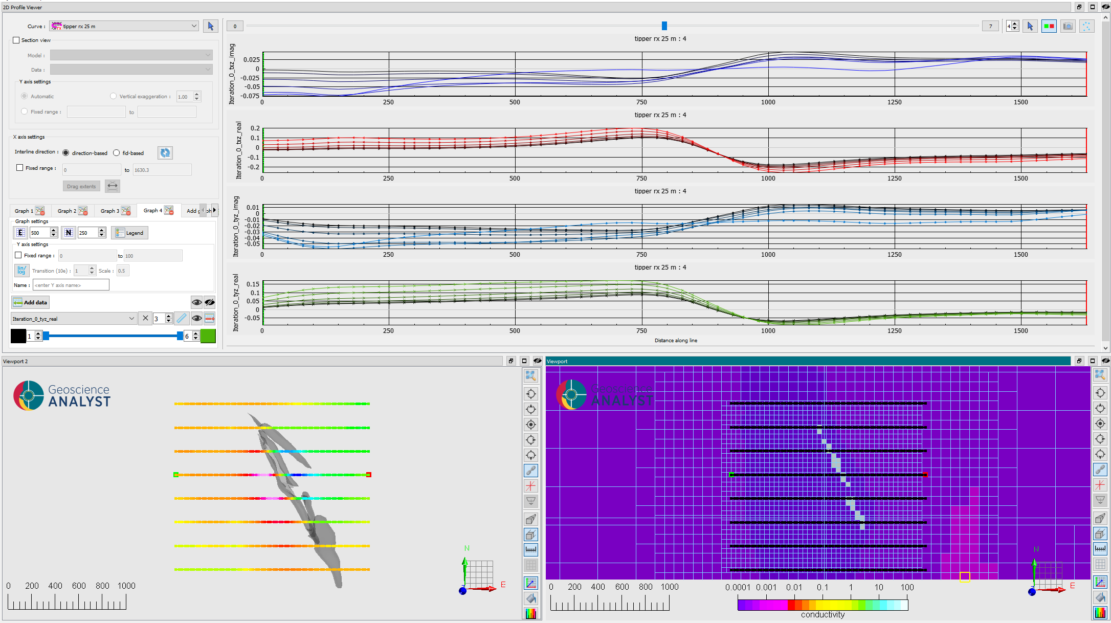
Fig. 29 (Top) Tipper data displayed by the 2D Profiler at all 6 frequencies for the 4 components (\(T_{zx}\), \(T_{zy}\), real and imaginary). (Bottom) Survey lines relative to (left) the ore body and (right) the discrete conductivity model.#
Note that the position of the known conductor correlates with large gradients in the tipper data.
Mesh creation#
In preparation for the inversion, we create an octree mesh optimized for the tipper survey. The mesh parameters are based on the original Flin Flon model.
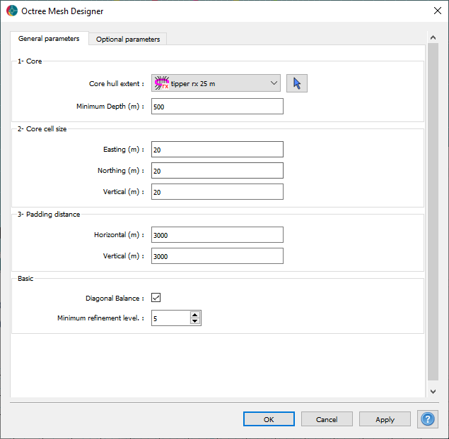
Fig. 30 Core mesh parameters.#
Note that the padding distances are set substantially further than for the magnetics, gravity or dc-resistivity (1 km) inversions. This is because the diffusion distance for a background resistivity of \(1000 \; \Omega .m\) for the lowest frequency (30 Hz) is roughly 3 km. This distance is important to satisfy the boundary conditions of the underlying differential equations.
Refinements#
For the first refinement, we insert 4 cells for the first three octree levels along the flight path. The refinement is done radially around the segments of the flight path curve to assure good numerical accuracy near the receiver locations. This is especially important for EM methods with low frequencies.
We use a second refinement along topography to get a coarse but continuous air-ground interface outside the area or interest.
Lastly, we refine a “horizon” to get a core region at depth with increasing cell size directly below the survey. This is our volume of interest most strongly influenced by the data.

Fig. 31 Refinement strategy used for the tipper modeling.#
See Mesh creation section for general details on the parameters.
Unconstrained inversion#
Runtime: ~2.0 h
Tipper data involves 2 receiver configuration (x and y), with two components (real and imaginary) and measured over 6 frequencies. Balancing all this data can be challenging and time consuming. Here we adopt a variable floor strategy based on the 10th percentile of each data layer.
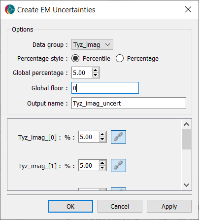
This approach is a good starting point, but experimentation is generally required.
After running the inversion we recover the following solution:
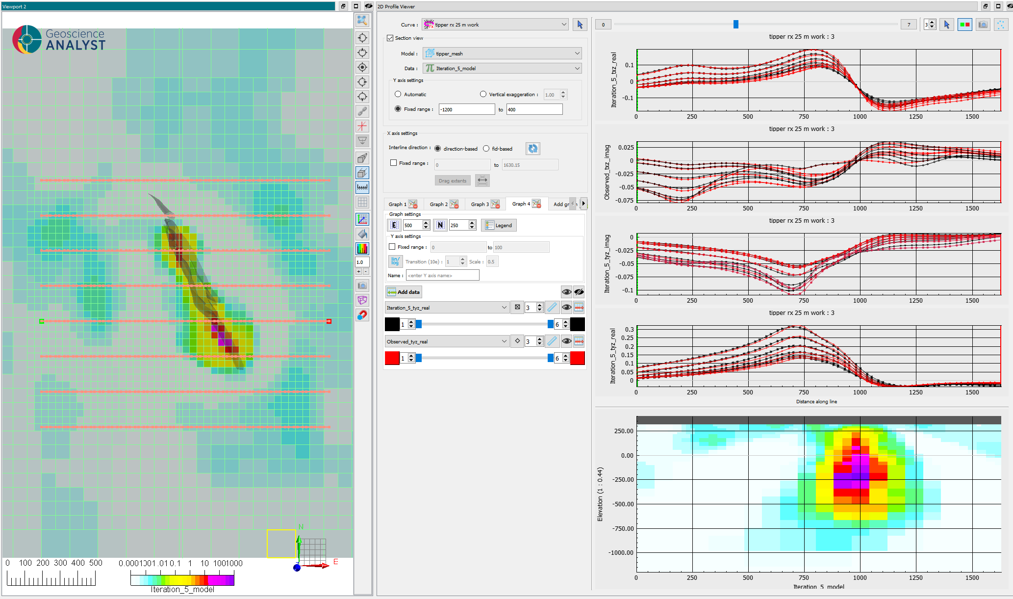
Fig. 32 (Left) Horizontal section at 120 m elevation after reaching target misfit (iteration 5).#
(Right)(top) 2D profiles of observed versus predicted data for all 4 channels and 6 frequencies and (bottom) vertical section through the conductivity model below the same line.
Despite our simplistic floor uncertainties, the inversion managed to converge fairly quickly to a reasonable model that fits our data well. We have recovered a clear conductor at depth that overlaps with the ore body. However, the inversion could not resolve the thin conductive overburden layer, as expected by the low frequency range of the tipper system.