Forrestania: Joint grav/mag

This case study focuses on the standalone and joint inversion of airborne magnetic data and synthetic gravity data. The magnetic data were downloaded from the Geoscience Australia GADDS Portal, while the gravity data were generated via forward modelling specifically for this exercise based on a derived iso-shell from magnetic inversion results. We cover the following steps:

• Data imports and pre-processing

• Standalone inversion of gravity data

• Standalone inversion of magnetic data

• Joint cross-gradient inversion

• K-means clustering analysis

Note

The following sections show how to run the same process using only open-source packages

• Gravity

• Magnetics

Authors
Glenn Pears	glennp@mirageoscience.com
Polyanna Rowe	polyannar@mirageoscience.com
Dominique Fournier	dominiquef@mirageoscience.com

Geological setting

The Forrestania Greenstone Belt, located in the Youanmi Terrane of the Eastern Yilgarn Craton, is known for its significant Ni-Cu-PGE mineralisation, primarily hosted within komatiitic units (Frost, 2003; Collins et al., 2012).

The belt features a structurally complex architecture, including:

• Synclines

• Faults

• Shear zones
  …that play a major role in sulphide localisation.

It is:

• Bounded by granitic and gneissic basement

• Intruded by monzogranite and granodiorite

• Transected by Proterozoic dolerite dykes (Perring et al., 1995)

Multiple deformation events have remobilised nickel sulphides into:

• Footwall sediments

• Granitic intrusions

→ Resulting in both typical (ultramafic-hosted) and atypical (granite-hosted) mineralisation (Collins et al., 2012).

---

The study area is largely underlain by granitic basement, adjacent to the Parker-Range–Hatters Hill greenstone belt to the east.

This north–south-trending belt is the regional host of:

• Nickel sulphide deposits in narrow ultramafic units

• Hosted within Archaean metabasalts and sulphidic sediments

🟡 Nearby deposits include:

• Beautiful Sunday

• Flying Fox

• New Morning

---

A prominent magnetic anomaly, trending E-W to ENE-WSW, is located just west of the greenstone belt.
Its:

• Strong magnetic response

• Orientation

• Coincident nickel-in-soil geochemistry

…suggest the presence of a mafic intrusion, making it a key geophysical target.

Fig. 40 Figure: Magnetic anomaly near the Greenstone belt interpreted as a potential mafic intrusion.

Data

Download the data package here

We first need to consolidate the data into a usable format. We use Geoscience ANALYST to import and convert the original files into the geoh5 format. The data bundle includes

• Airborne magnetic survey: 60472_AOI4.gdb

• Ground gravity survey: Forrestania_Gravity_Station_trim_.csv Note: this is a synthetic dataset generated for inversion testing purposes.

• Digital Elevation Model (DEM): Forrestania_SRTM1 Australia_MGA50.ers

This can be done with a simple drag & drop to the viewport, or one at a time through the import menu. Once imported, the data can be activated for visualization.

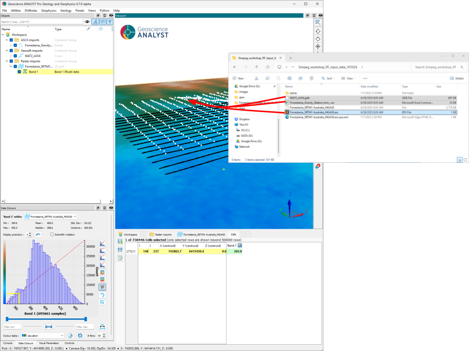
Fig. 41 Data imported from their original format to geoh5 for visualization.

Processing

Note that both the DEM and airborne magnetic survey were imported at an arbitrary 0 m elevation and do not reflect the true position. We first need to modify our object such that the data is accurately located in 3D space.

Step 1: Convert the 2D DEM into a 3D surface

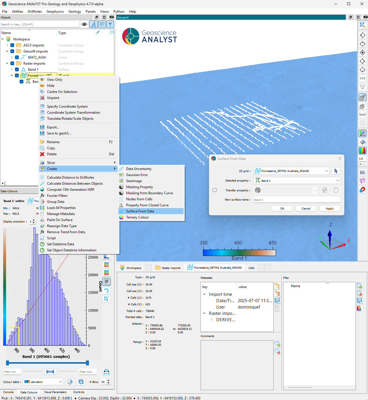
Fig. 42 [Click to enlarge]

Step 2a: Transfer the DEM data onto the airborne survey (curve).

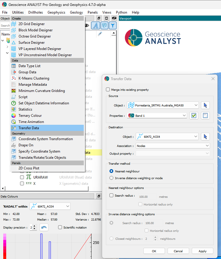
Fig. 43 [Click to enlarge]

Step 2b: Re-assign the Z channel to the DEM + radar height.

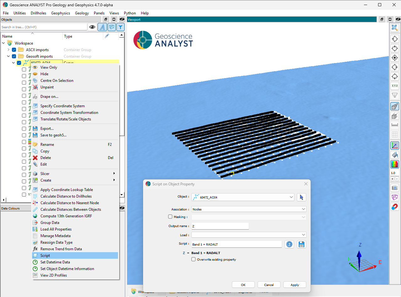
Fig. 44 [Click to enlarge]

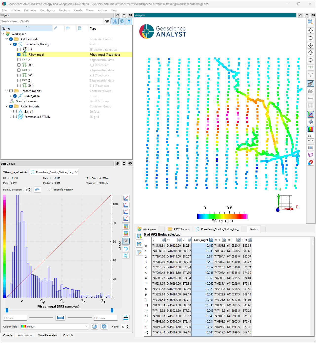
Gravity

We begin our analysis with the gravity dataset. As the publicly available ground gravity data in this region do not have the resolution required to image the target anomaly, we used synthetic data for this exercise.

The gravity response was generated by forward modelling an iso-shell derived from one of the completed magnetic inversion models. Random noise were added to make the synthetic dataset more realistic and challenging for inversion.

Inputs

Gravity data are sensitive to variations in the density of rocks. The gravity dataset, being synthetic, was generated in the form of terrain-corrected (2.67 g/cc) residual data. We can therefore proceed directly to the inversion phase.

Inversion options

The following options are set for the inversion.

Fig. 45 [Click to enlarge]

• Assign the data uncertainty to a quarter of the standard deviation (0.05 mGal). This is a somewhat conservative estimate that takes into account both the instrumental and numerical noise.

• Use a 0 g/cc reference value for the model. This assumes that the signal from the background density was accurately subtracted from the data.

• Leave the Mesh option unchecked. We will let the code create an octree mesh based on the average data separation and extent.

Results

After completion of the inversion, we load the results and assess convergence and data fit.

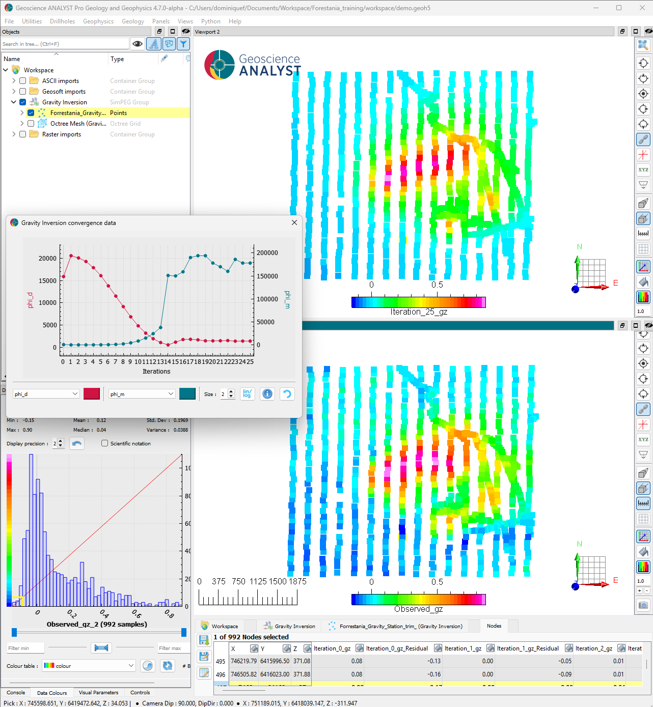
We note the following:

• It took 13 iterations to converge to the target misfit.

• The following 12 iterations have increased the model complexity (\(phi_m\)) but preserved the data fit (\(phi_d\)).

• Most of the important gravity anomalies appear to be reproduced by the final model.

Smooth solution (L2-norm)

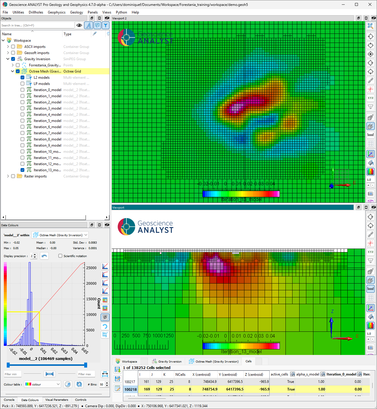
The smooth solution (iteration 13) indicates the presence of a dense anomaly extending at depth with density contrasts ranging from [-0.02, 0.05] g/cc. The negative density contrasts appear to be localized around the main positive anomaly, likely due to the smoothness constraint and the lack of bound constraints. Some smaller “fuzzy” anomalies are visible at the margins.

Compact solution (L0-norm)

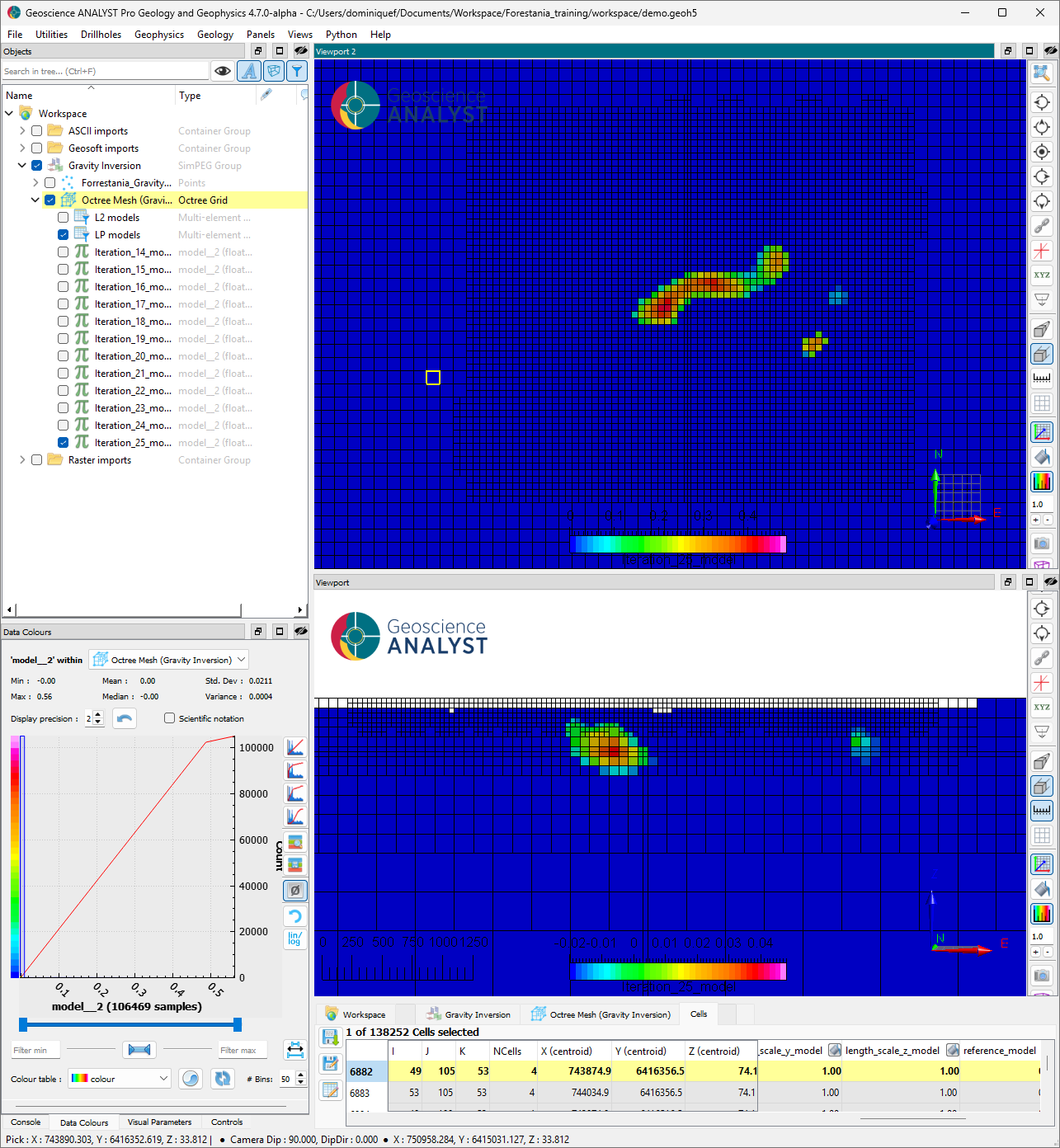
As an alternative solution, the compact model (iteration 25) recovers a well-defined dense body within a mostly uniform background. Density contrasts have substantially increased in the range of [0.0, 0.56] g/cc.

Magnetics

We follow up with the processing of the airborne magnetic data.

Inputs

The source of the magnetic signal can generally be attributed to the presence or destruction of magnetic minerals in rocks (mainly magnetite). Magnetometers measure the Total Magnetic Intensity (TMI), which includes both the primary (source) field and secondary fields (signal) from the local geology.

Step 1: Residual data

The inversion routine requires Residual Magnetic Intensity (RMI). The first step is to compute and remove the primary field (IGRF) at the time and location of acquisition. The survey was conducted between February and March 1988.

Step 1a: Set the coordinate system of the survey

Before computing the IGRF, we need to locate the survey in world coordinates. This specific project is referenced to the MGA zone 50 coordinate system.

Fig. 46 [Click to enlarge]

Step 1b: Lookup/remove IGRF

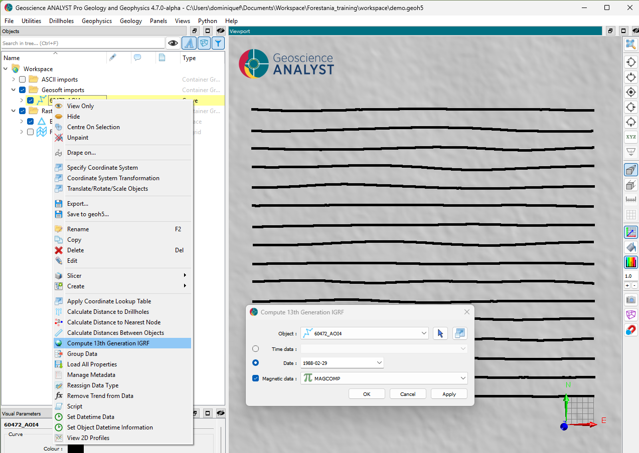
Fig. 47 [Click to enlarge]

The inducing field parameters at the time and location of the survey are:

Magnitude: \(59127\) nT

Inclination: \(-66.9^\circ\)

Declination: \(-1.05^\circ\)

Step 2: Detrend

The local background field appears to be slightly lower (~112 nT) than the computed IGRF model, as most of the data away from the main anomaly are below 0. To avoid modelling this background trend, we can remove the median value.

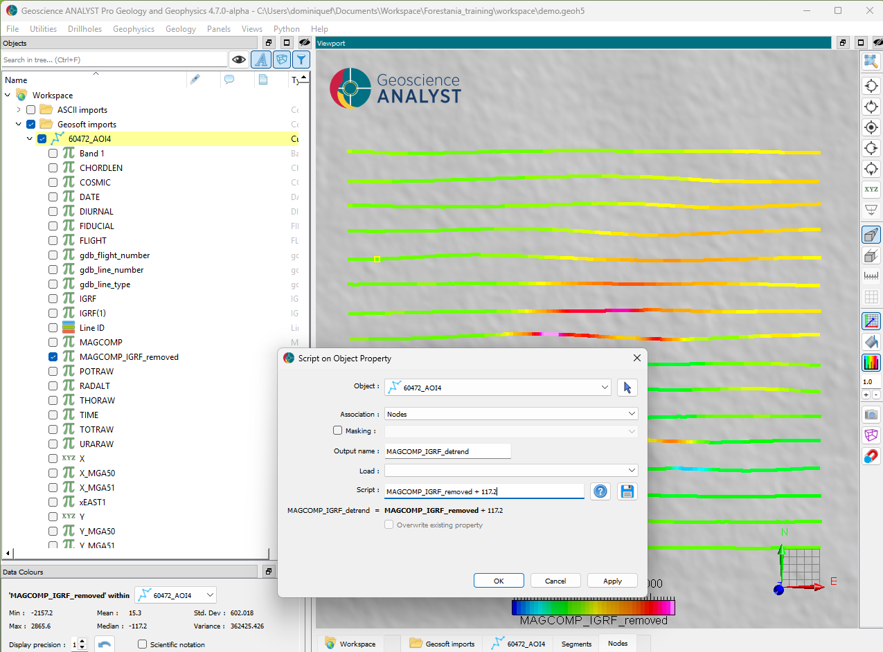
Fig. 48 [Click to enlarge]

Step 3: Downsampling

We can downsample the data along lines to reduce the computation cost of the inversion. Since the average flight height of this survey was 60 m, we can confidently downsample the lines by the same amount without affecting the wavelengths contained in the data.

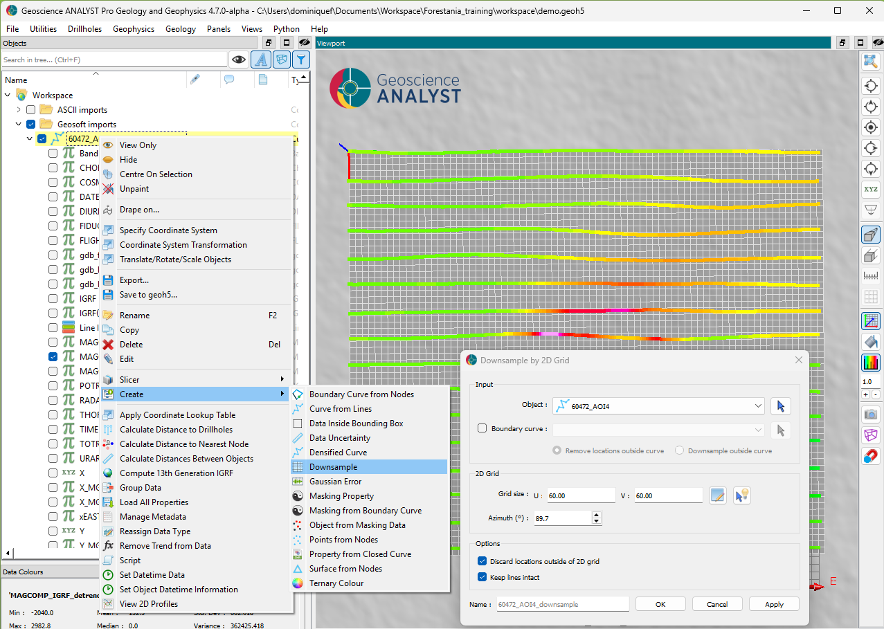
Fig. 49 [Click to enlarge]

Create a mesh

This time, we will create a mesh using the Octree Mesh Creation application. In preparation for the joint inversion, we will simply modify the gravity mesh parameters. By doing so, we guarantee that the extent and base cell size remain the same, only the refinements will be optimized to the magnetic survey.

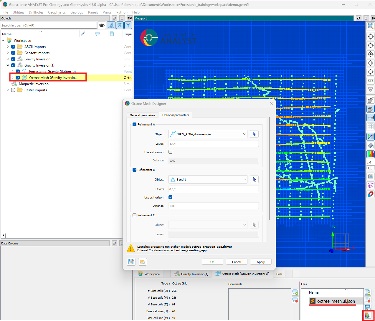
Step 1: Load the octree parameters

Inspect the files attached to the gravity mesh object and load the ui.json.

Step 2: Modify the refinements

Change the input object for Refinement A for the curve object of the magnetic survey.

Step 3: Run and load the results

Inversion options

The following options are set for the inversion.

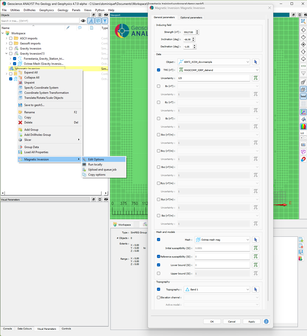
Fig. 50 [Click to enlarge]

• Set the inducing field parameters as described above.

• Assign the data uncertainty to a quarter of the standard deviation (125 nT).

• Use a 0 SI reference value for the model. This assumes that we removed all background signal from the data.

• Assign the newly created octree mesh object.

• Leave the default lower bound value to 0 SI (non-negative).

Results

After completion of the inversion, we load the results and assess convergence and data fit.

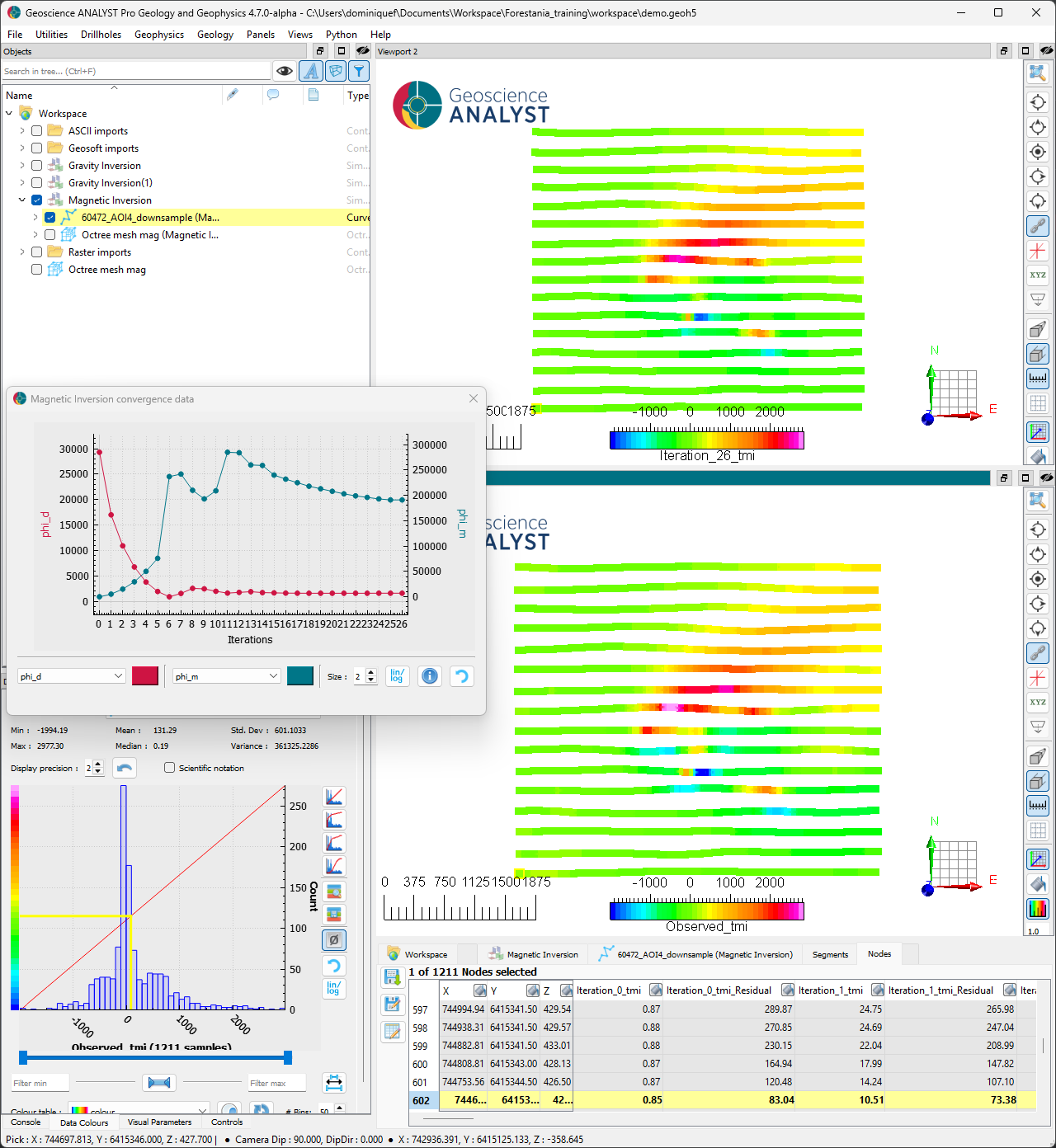
We note the following:

• It took 5 iterations to converge to the target misfit.

• The following 21 iterations have increased the model complexity (\(phi_m\)) while preserving the data fit (\(phi_d\)).

• Small anomalies are under-fitted, which could warrant a second inversion with lower uncertainties.

Smooth solution (L2-norm)

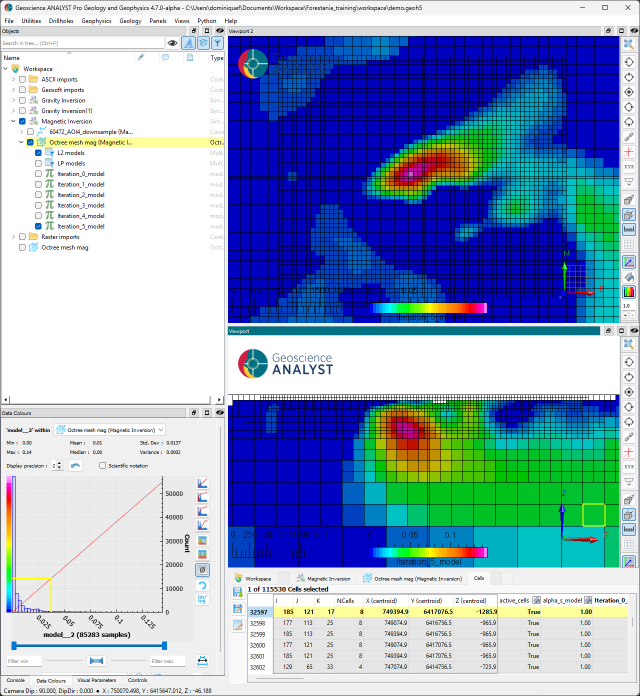
The smooth solution (iteration 5) indicates the presence of a susceptible body at depth. The shape and location of the anomaly resemble the solution obtained with the gravity modelling, including the presence of smaller “fuzzy” anomalies at the margins.

Compact solution (L0-norm)

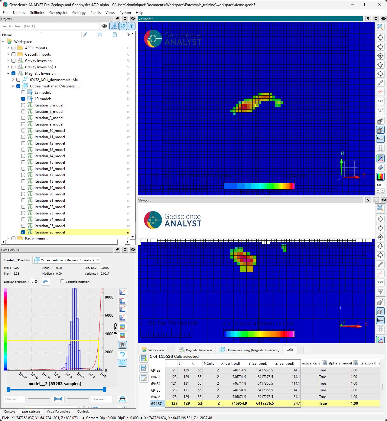
As an alternative solution, the compact model (iteration 21) recovers a well-defined dense body within a mostly uniform background. Susceptibility contrasts have substantially increased in the range of [0.0, 2.0] SI.

Joint cross-gradient

After inverting the gravity and magnetic data independently, and recovering anomalies with similar shapes and positions in both, the next step is to invert both datasets jointly. We are going to employ the cross-gradient constraint to promote alignment of edges in the density and susceptibility models.

Inversion options

The following options are set for the inversion.

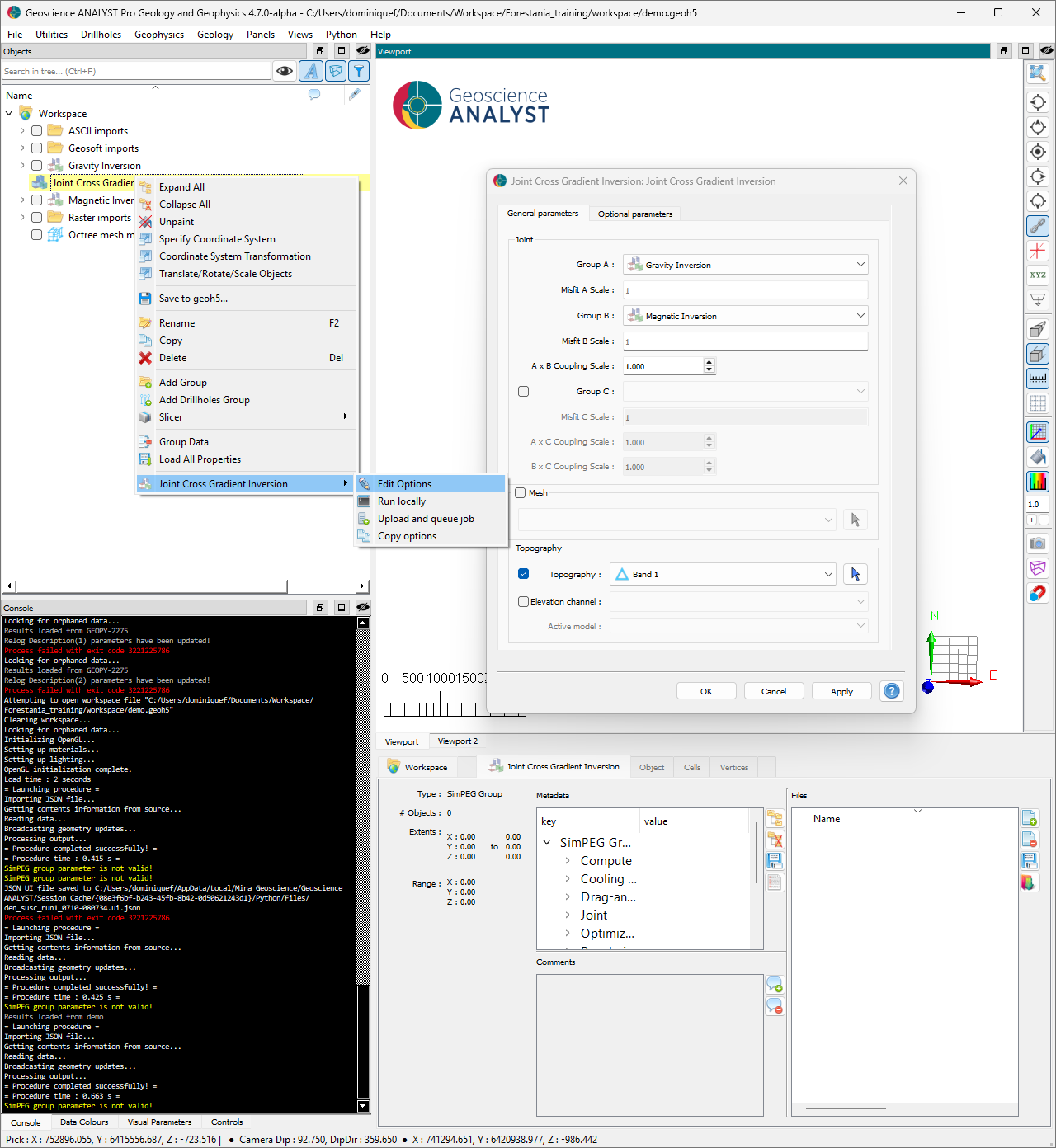
Fig. 51 [Click to enlarge]

• Select the two existing inversion groups (magnetic and gravity) to Group A and B.

• Leave the mesh option empty. The routine will generate an inversion mesh based on the best resolution from both the gravity and magnetic problems.

• Set the topography

Results

After completion of the inversion, we load the results

We note the following:

• The shape of the density and magnetic susceptibility models match closely near the main anomaly.

• Some of the smaller anomalies, as well as an extension to the north-east, are only seen in the density model.

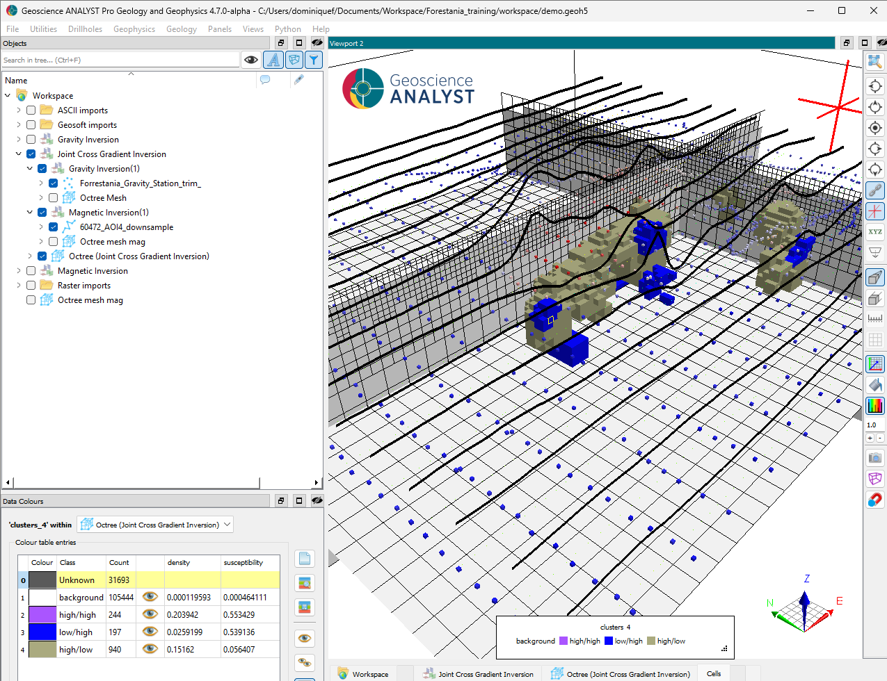
Analysis

The joint inversion results highlight a few features that could be distinguished by their physical property contrasts. After running a K-means clustering on the final models, we recover the following simplified petrophysical model with 4 units.

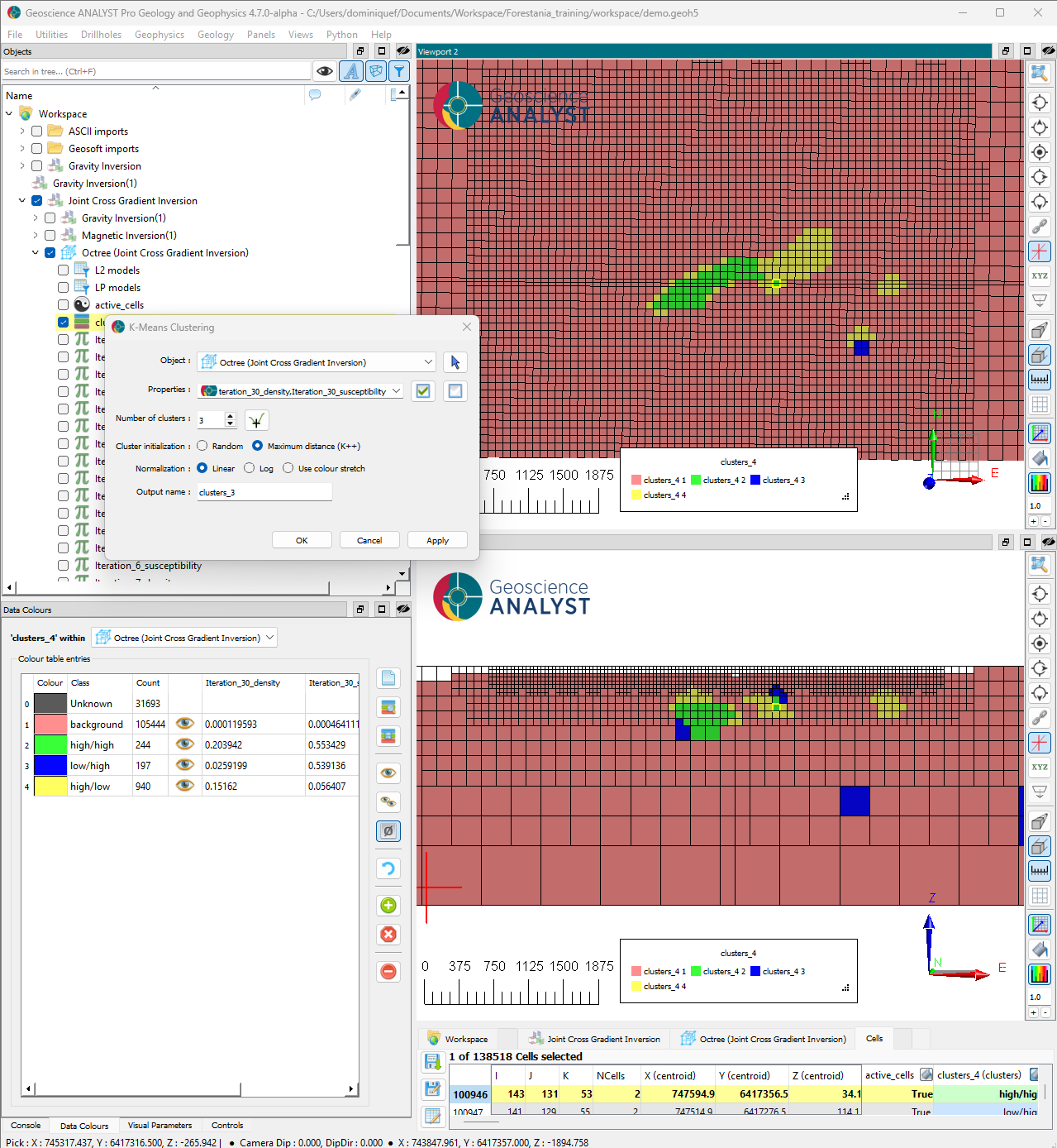
This table summarizes the different units based on their mean density and susceptibility values.

Table 2 Summary of expected physical properties

Unit	Susceptibility	Density
background	low	low
A	high	high
B	low	high
C	high	low

Summary

• We have inverted publicly available data over the Forrestania geological province.

• The joint cross-gradient method was successful in promoting similarities between the different physical properties wherever possible.

• Our results suggest the presence of different geological units with distinct density and magnetic susceptibility signatures.

References

Collins, J. E., Hagemann, S. G., McCuaig, T. C., & Frost, K. M. (2012). Structural controls on sulfide mobilization at the high-grade Flying Fox Ni-Cu-PGE sulfide deposit, Forrestania Greenstone Belt, Western Australia. Economic Geology, 107(7), 1433–1455. https://doi.org/10.2113/econgeo.107.7.1433

Frost, K. M. (2003). Geology and nickel sulfide deposits of the Forrestania Greenstone Belt, Western Australia. Mineralium Deposita, 38(6), 648–663.

Perring, C. S., Barnes, S. J., & Hill, R. E. T. (1995). The Widgiemooltha dike suite: Geochemistry, emplacement, and implications for the evolution of the Eastern Goldfields Province, Western Australia. Australian Journal of Earth Sciences, 42(5), 489–502.