Depth of Investigation

This application allows users to compute a depth of investigation from model values. In geophysics, “depth of investigation” refers to the maximum depth below the surface from which a geophysical survey can reliably measure. It depends on factors like the survey design and physical properties of the subsurface material.

Several strategies have been proposed to assess uncertainties in models recovered from inversion. Nabighian and Macnae [NM89] used a skin depth approach for electromagnetic surveys, assuming a background halfspace resistivity. Li Y. and Oldenburg [LYO99] implemented a cut-off value based on two inverted models obtained with slightly different assumptions.

This application uses the method proposed by A.V. and E. [AVE12], based on the sum-square of sensitivities to estimate a volume of low confidence.

Interface

The depth of investigation methods based on sensitivity cutoffs relies on the ui.json interface.

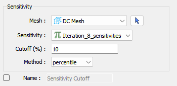
Inputs

• Mesh: The mesh used for inversion

• Sensitivity: Model selector for the sensitivities at a given iteration (see Pre-requisite)

• Cut-off: Percentage value to threshold the sentivities, relative to the Method used.

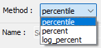
• Method: One of percentile, percent or log percent

Output

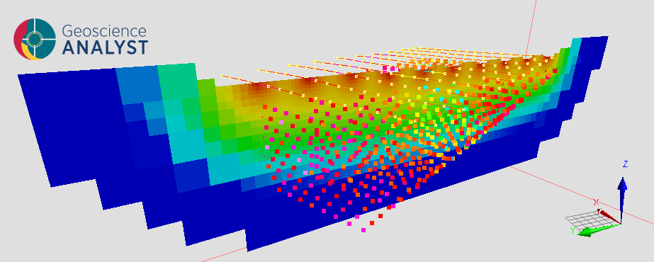
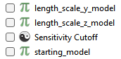
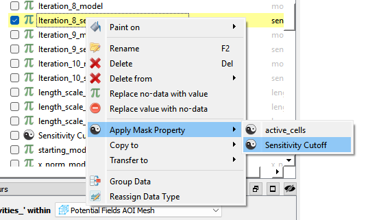
After running, the application will create a masking attribute saved on the mesh.

The mask can then be applied to any of the iterations to show only the cells that exceeded the sensitivity threshold.

Pre-requisite

In order to save the sensitivities during a SimPEG inversion, the ‘Save sensitivities’ option must be selected from the ‘Optional parameters’ tab of an inversion.

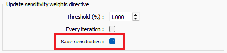
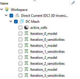
This will result in a new model generated and saved into the computational mesh at each iteration.

Methodology

The sensitivity matrix is calculated as part of the optimization problem solved by SimPEG while inverting geophysical data. The sensitivity matrix represents the degree to which each predicted datum changes with respect to a perturbation in each model cell. It is given in matrix form by

\[ \mathbf{J} = \frac{\mathbf\partial{F}(\mathbf{m})}{\partial{\mathbf{m}}} \]

where \(\mathbf{m}\) is the model vector, and \(F(\mathbf{m})\) represents the forward modelling operation as a function of the model. The sensitivity matrix \(\mathbf{J}\) is a dense array with dimensions \(N\times M\), where \(N\) is the number of data and \(M\) are the number of mesh cells.

The depth of investigation mask is a property of the cells of the mesh only so the rows of the sensitivity matrix (data) are sum-square normalized as follows.

\[ \|\mathbf{j}\| = \left[\sum_{n=1}^{N}\left(\frac{\mathbf{J}_{n:}}{w_n}\right)^{2}\right]^{(1/2)} \]

where \(w_n\) are the data uncertainties associated with the \(n^{th}\) datum.

The resulting vector \(\|\mathbf{j}\|\) can then be thought of as the degree to which the aggregate data changes due to a small perturbation in each model cell. The depth of investigation mask is then computed by thresholding those sensitivities

Thresholding

The depth of investigation can be estimated by assigning a threshold on the sum-squared sensitivity vector. This can be done as a percentile, percentage, or log-percentage. In the percentile method, the mask is formed by eliminating all cells in which the sensitivity falls below the lowest \(n\)% of the number of data where \(n\) is the chosen cutoff. In the percent method the data are transformed into a percentage of the largest value

\[ d_{scaled} = \frac{100 \cdot d}{max(d)} \]

and the mask is formed by eliminating all cells in which the sensitivity falls below the lowest \(n\)% of the data values where \(n\) is the chosen cutoff. Finally, the log-percent mask transforms the data into log-space before carrying out the percentage thresholding described above.