Rotated Gradients

This section provides details about rotating the model gradients used in the Regularization function. When applied in conjunction with weights and sparse norms, the rotation helps reinforce structural trends, as depicted in the image below.

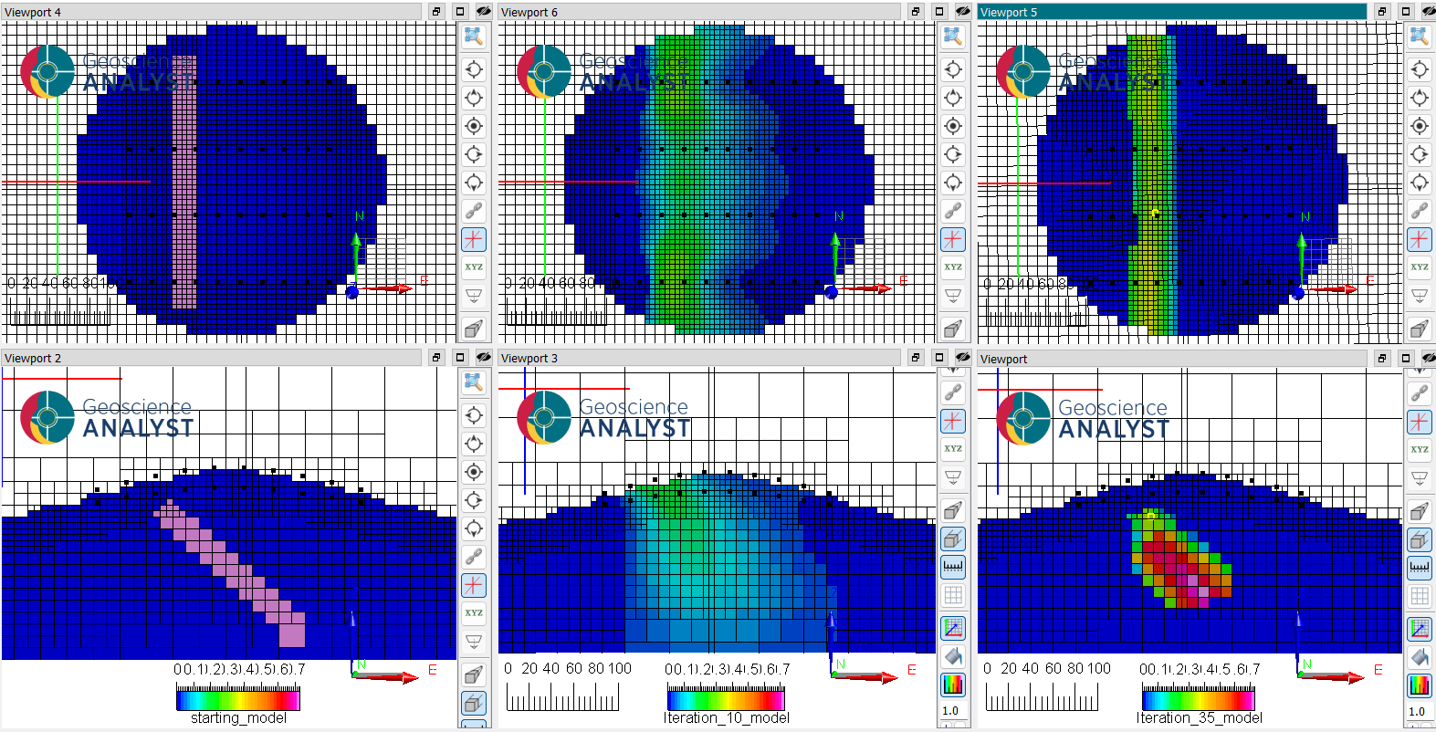
Fig. 1 (Top) Horizontal and (bottom) vertical sections through (left) a simple dipping dyke model under smooth topography. (Center) Model recovered using the conventional smooth norm inversion. (Right) Compact model obtained with a dip rotation of \(45\\circ\) towards East.

Rotation angles can be applied globally or on a cell-by-cell basis to reflect local orientations, such as faults and folds.

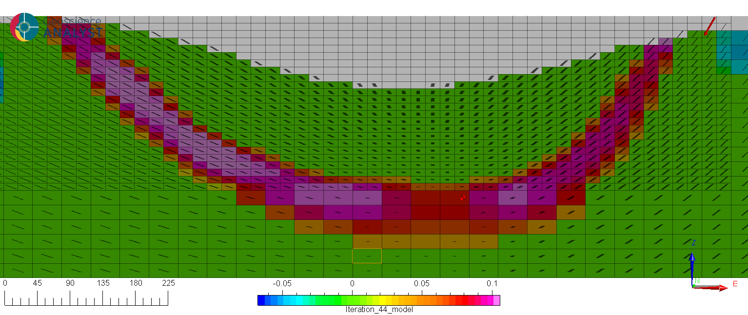
Fig. 2 Example of an inversion with local rotations along the expected limbs of a folded layer.

Input format

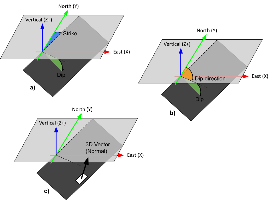
Direction information must be supplied as a Data Group defined on the inversion mesh. The following group types are accepted: Dip direction & Dip, Strike & Dip, or 3D vector.

The dip angles (degrees) are positive downward from the horizontal. The strike and dip direction angles (degrees) are positive clockwise from North. The 3D vector data defines the unit normals, which are perpendicular to both the Dip direction & Dip and Strike & Dip directions. As illustrated below, all three formats define a rotated plane in 3D.

Background

As covered in the Model Smoothness section, penalties on the model gradients are measured by:

\[ \mathbf{f}_i = \mathbf{G}_i (\mathbf{m} - \mathbf{m}_{ref}), \]

where \(\mathbf{G}_i\) is a finite difference operator that computes the difference in model \(\mathbf{m}\) values between adjacent cells along one of the Cartesian directions: East (X), North (Y), and vertical (Z). As proposed by Li. and Oldenburg [LiO00], orientation information can be incorporated into the inversion by rotating the gradient operators along arbitrary directions such that

\[ \mathbf{\hat f}_i = \mathbf{\hat G}_i (\mathbf{m} - \mathbf{m}_{ref}), \]

where \(\mathbf{\hat G}_i\) are rotated gradients along one of the \(u\), \(v\), and \(w\)-axes.

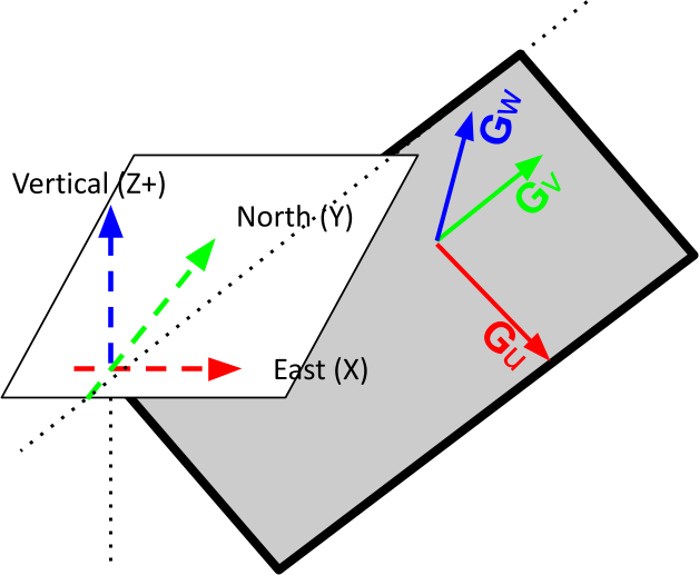
Fig. 3 Rotation of the Cartesian axes along an arbitrary plane.

• \(X \rightarrow u\) pointing down-dip

• \(Y \rightarrow v\) pointing along strike

• \(Z \rightarrow w\) pointing along the normal

Simpeg-Drivers uses a combination of both forward and backward gradient operators to achieve better symmetry in 3D. The gradient operators are constructed based on the partial volumes intercepted by ghost cells rotated about the center of each cell. The partial volumes include all diagonal neighbours intercepted by the ghost cells.

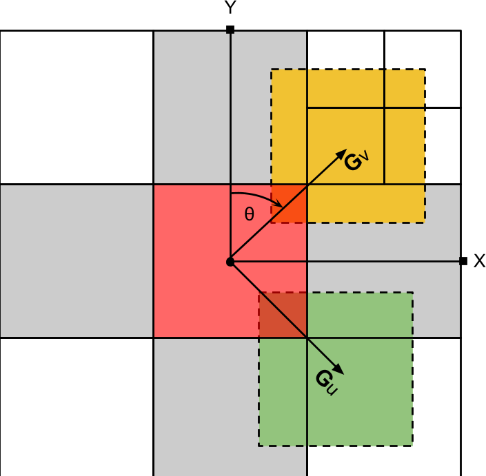
Fig. 4 Plan-view depiction of the \(u,v\) forward gradient operators, made up of partial volumes from neighbouring cells.

The full regularization term is made up of seven terms in total:

\[ \phi_m = \| \mathbf{W}_s (\mathbf{m} - \mathbf{m}_{ref}) \|_2^2 + \sum_{i = u^F,v^F,w^F} \| \mathbf{W}_i \mathbf{G}_i(\mathbf{m}) \|_2^2 + \sum_{i = u^B,v^B,w^B,} \| \mathbf{W}_i \mathbf{G}_i(\mathbf{m}) \|_2^2 \]

Example

This example demonstrates the use of rotated gradients on a semi-realistic synthetic model. The geometry of the model mimics a banded-iron formation buried under a hill. The goal is to demonstrate the benefit of applying directional constraints to the inversion to better resolve dipping anomalies.

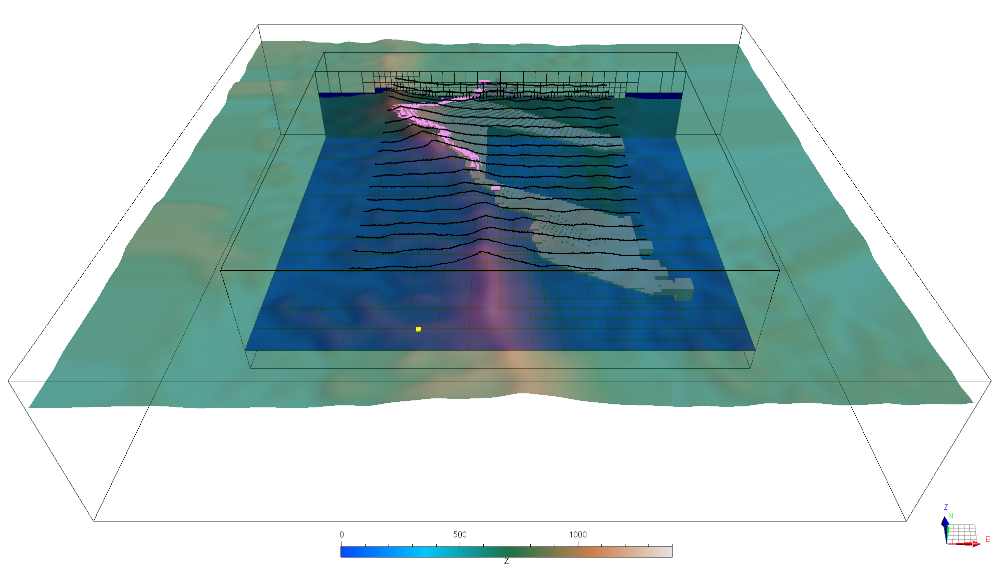
Fig. 5 Synthetic model consisting in a folded dipping magnetic layer.

The model comprises a folded and faulted magnetic layer (0.5 SI) dipping 20 degrees towards the east. The model was generated using several structural control points provided to the Gempy application.

From this model, residual magnetic field data were simulated along an East-West survey with 200 m line spacing and a mean terrain clearance of 150 m. For simplicity, a vertical inducing field with a magnitude of 50,000 nT was used.

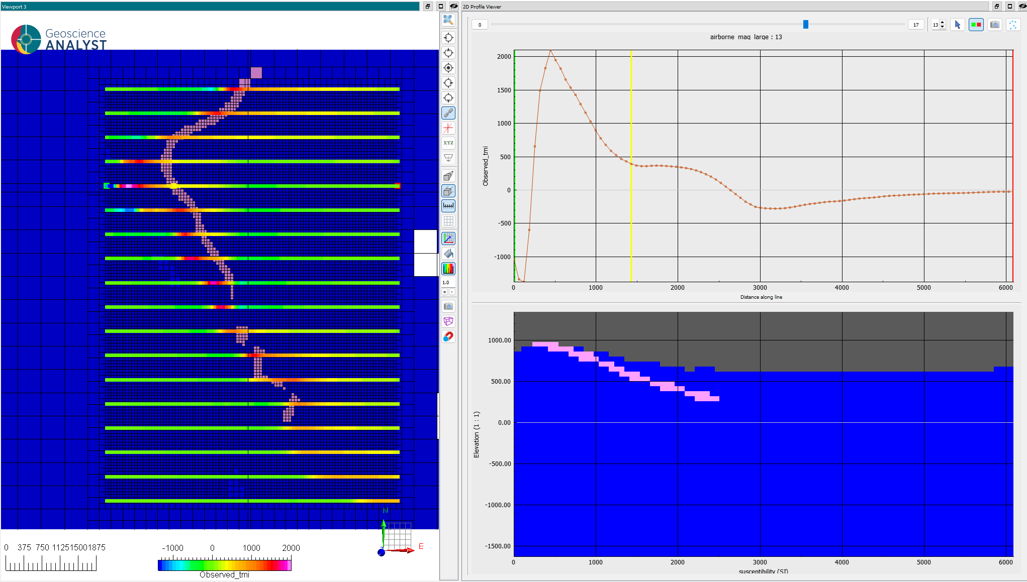
Fig. 6 (Left) Horizontal section through the discrete model overlaid by the TMI data. (Right) Vertical section through the model and (top) TMI data profile.

The basic components (data, model, and topography) to reproduce this example can be downloaded here.

Unconstrained inversion

As a starting point, the magnetic data were inverted with standard constraints (lower bounds and reference value of 0 SI).

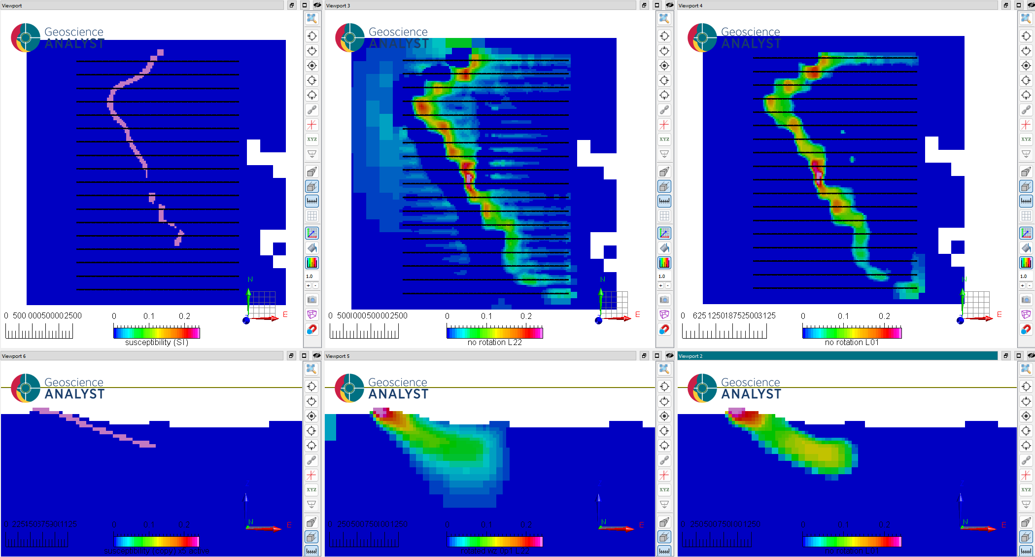
Fig. 7 (Top) Horizontal and (bottom) vertical sections through the (left) true, (middle) inverted-smooth and (right) recovered inverted-compact model without using rotated gradients.

The resulting model shows clumping of the magnetic anomalies around the survey lines. This is expected from an unconstrained inversion, as the regularization function dominates in regions of low sensitivity, smoothing and lowering the susceptibility values away from the receiver locations. The shape and dip of the magnetic layer become even more diffuse at depth. The subsequent compact model only slightly improves the results by shrinking the volume of the magnetic highs, but fails to improve the geometry of the layer.

Directional constraints

To improve the continuity of the magnetic layer across lines and down-dip, trend information from the structural control points was provided to the inversion.

First, the dip and dip-direction data from the structural markers were interpolated to the inversion mesh using the Radial Basis Function (RBF) application. Following the instructions presented in the previous section, the interpolated data were grouped as type Dip Direction & Dip. Users can then validate the constraints by displaying the vectors on sections of the mesh.

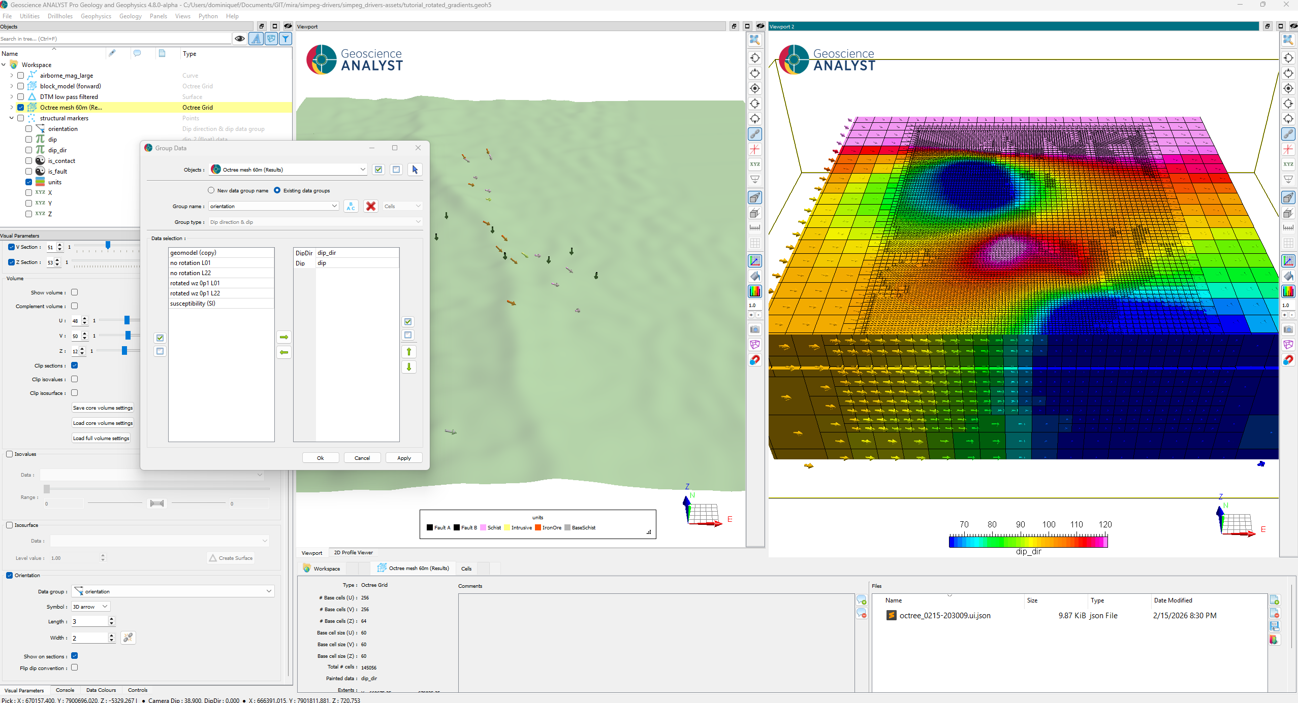
Fig. 8 (Left) Perspective view of the structural constraints with dip and direction. (Right) Interpolated dip and direction onto the inversion mesh, also group as Dip Direction & Dip for visualization and inversion.

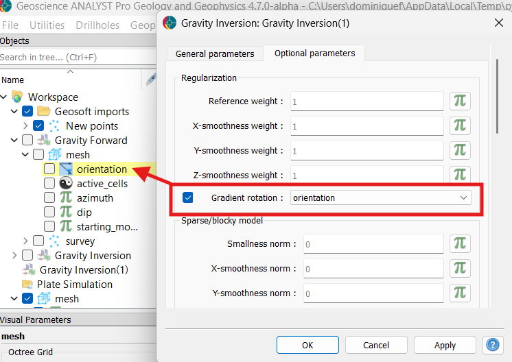
To further accentuate the trend, the weight of the Z-smoothness weight was decreased, as it is now oriented perpendicular to the plane of rotation. By doing so, the relative strength of the smoothing (and sparsity) along the local dip and strike of the magnetic layer is increased.

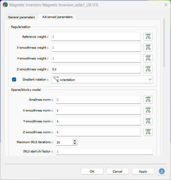
Fig. 9 Regularization parameters used for the sparse rotated gradient inversion.

After reaching the target misfit, both the smooth and sparse models show a clear improvement in resolving a continuous magnetic layer. In cross-section, the dip and thickness of the layer are significantly improved at depth, although the dip angle is slightly overestimated.

Note that a similar strategy could have been to increase both the X and Y-smoothness weight. This, however, would implicitly underweight the penalty on the reference model, yielding an overall smoother model.

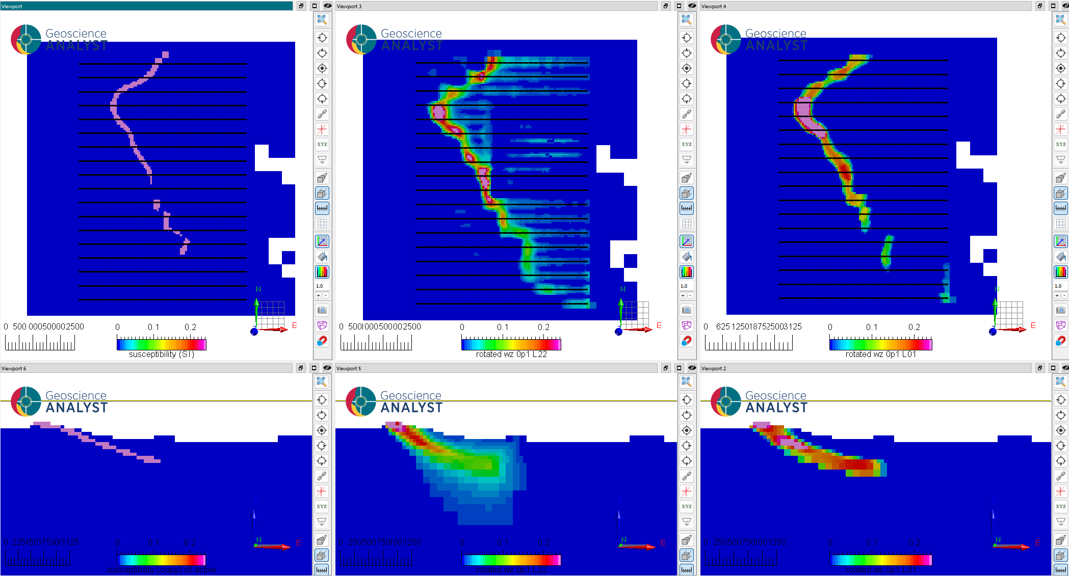
Fig. 10 (Top) Horizontal and (bottom) vertical sections through the (left) true, (middle) inverted-smooth and (right) recovered inverted-compact model with rotated gradients.