
Model constraints#
This section focuses on model constraints, or regularization functions, that can inject “geological knowledge” into the inversion process. More specifically, this section covers the weighted least-squares regularization functions. Readers are invited to visit the following sections for more advanced options
Least-squares regularization#
The conventional L2-norm regularization function imposes constraints based on least-squares measures, either of the model and/or its spatial gradients.
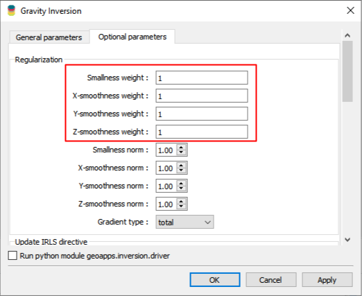
For 3D inverse problems, the full regularization function contains 4 terms: one for the reference model and three terms for the smoothness measures along the three Cartesian axes. We can express these various constraints as
Weighting matrices \(\mathbf{W}_i\) are added to each function to scale the constraints among each other. While often referred to as an unconstrained inversion, one could argue that the conventional least-squares regularization does still incorporate first-degree information about the geological background, at least in the form of physical property distribution. The following sections provide details on each element of the regularization.
Model smallness (reference)#
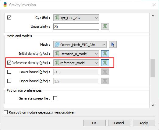
In the seminal work of Tikhonov et al. [TASY95], the function \(f(\mathbf{m})\) simply measures the deviation between the inversion model from a reference value
where \(\mathbf{m}_{ref}\) is a reference model. This function tries to keep the model “small”, in terms of deviation from the reference values. The reference model can vary in complexity, from a constant background value to a full 3D geological representation of the physical property.
Model smoothness (gradients)#
A second set of terms can be added to the regularization function to apply constraints on the model gradients, or the roughness, of the solution. Following the notation used in Li. and Oldenburg [LiO98],
where \(\mathbf{G}_i\) is a finite difference operator that measures the gradient of the model \(\mathbf{m}\) along one of the Cartesian directions. Three functions are needed to calculate the model gradients along the Easting (\(f_x\)), Northing (\(f_y\)) and vertical (\(f_z\)) directions. These functions enforce the model to remain smooth, as large gradients (sharp contrasts) are penalized strongly.
Weights#
The diagonal weighting matrices \(\mathbf{W}_i\) are made up of default and user-defined weights
User-defined weights (\(\mathbf{w}_u\))#
User-defined weights can be tuned to emphasize the contribution of a
particular function. This can be done globally, as a constant, or
locally on a cell-by-cell basis.
Weights may reflect variable degrees of confidence in the reference geological model (e.g. high near the surface, low at depth), or to accentuate specific trends in the model.
Sensitivity-based weights (\(\mathbf{w}_s\))#
Sensitivity-based weights are computed as the sum-squares the rows of the sensitivities
where \(\mathbf{J}\) are the sensitivities (Jacobian) of the forward problem. The weighting attempts to compensate for the strong influence of the misfit function near the receiver locations, which would favour a model with high complexity near the surface. A small constant \(\epsilon\) is added to threshold the weights in regions of extremely low sensitivity.
Dimensionality scaling (\(\mathbf{w}_h\))#
Dimensionality scaling is applied to the gradient terms \(\phi_{i=(x,y,z)}\) as constants to account for length scales in the smoothness terms
where \(h\) is defined by the smallest cell dimension in each dimension \(i=x,y,z\). This default scaling brings the smallness and smoothness terms to be dimensionally equivalent, which would otherwise be