Sparse regularization

It is possible to generalize the conventional least-squares approach such that we can recover different solutions with variable degrees of sparsity. By sparsity, we mean fewer model cells (or gradients) away from the reference, but with larger values. The goal is to explore the model space by changing our assumption about the character of the solution, in terms of the volume of the anomalies and the sharpness of their edges. We can do this by changing the “ruler” by which we evaluate the model function \(f(\mathbf{m})\).

Smallness norm model

The first option is to impose sparsity assumptions on the model values.

\[ \phi(m) = \| (\mathbf{m} - \mathbf{m}_{ref} \|_p \;. \]

That is, we ask the inversion to recover anomalies that have small volumes but large physical property contrasts. This is desirable if we know the geological bodies to be discrete and compact (e.g. kimberlite pipe, dyke, etc.). The example below demonstrates the outcome of an inversion for different combinations of norms applied to the model

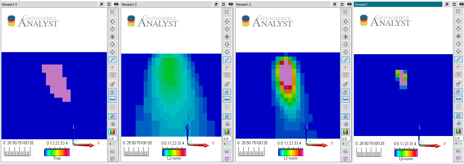The figure above shows vertical sections through the true and recovered models (from left to right) with L2, L1 and L0-norm on the model values.

Note that as \(p \rightarrow 0\) the volume of the anomaly shrinks to a few non-zero elements while the physical property contrasts increase. They generally agree on the center position of the anomaly but differ significantly in their extent and shape.

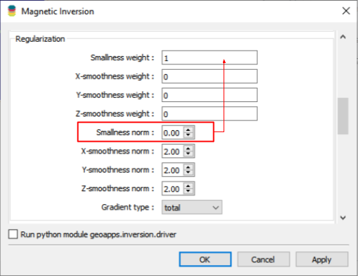
No smoothness constraints were used (\(\alpha_{x,y,z} = 0\)), only a penalty on the reference model (\(m_{ref} = 0\)).

All those models fit the data to the target data misfit and are therefore valid solutions to the inversion.

Smoothness norm model

Next, we explore the effect of applying sparse norms on the model gradients.

\[ \phi(m) = \| |\nabla \mathbf{m}| \|_p \]

or in matrix form

\[ \phi(m) = \| \sqrt{(\mathbf{G}_x \mathbf{m})^2 + (\mathbf{G}_y \mathbf{m})^2 + (\mathbf{G}_z \mathbf{m})^2} \|_p \;. \]

In this case, we are requesting a model that has either large or no (zero) gradients. This promotes anomalies with sharp contrast and constant values within.

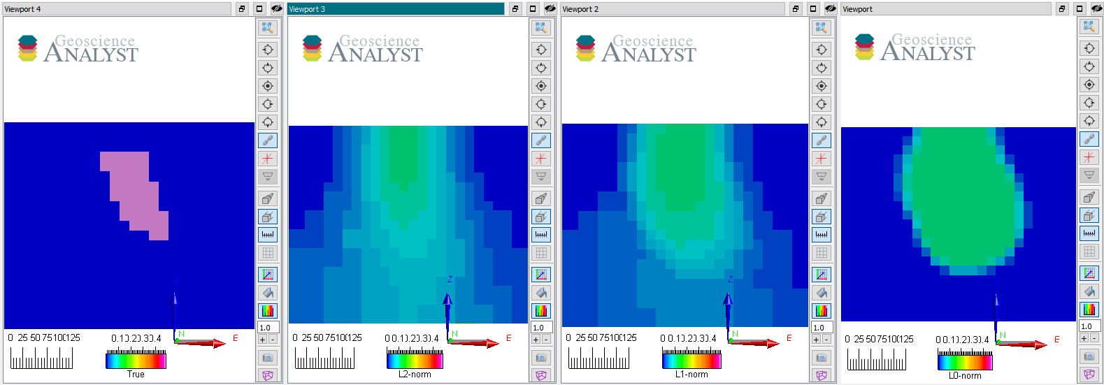The figure above shows vertical sections through the true and recovered models (from left to right) with L2, L1 and L0-norm on the model gradients.

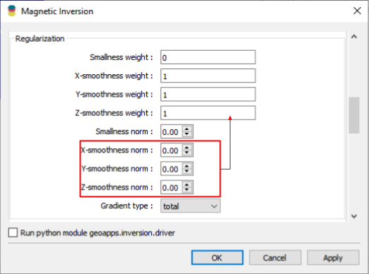
No reference model was used (\(\alpha_s = 0\)) with uniform norm values on all three Cartesian components.

All those models also fit the data to the target data misfit and are therefore valid solutions to the inversion. Note that as \(p \rightarrow 0\) the edges of the anomaly become tighter while variability inside the body diminishes. They generally agree on the center position of the anomaly but differ greatly on the extent and shape.

Mixed norms

The next logical step is to mix different norms on both the smallness and smoothness constraints. This gives rise to a “space” of models bounded by all possible combinations on \([0, 2]\) applied to each function independently.

To be continued…

Background: Approximated \(L_p\)-norm

The standard \(L_p\) norm measure is generally written as

\[ \phi(m) = \| f(\mathbf{m}) \|_p ] \;, \]

which can also be expressed as

\[ \phi(m) = \sum_{j}^M {|f(m)_i |}^p \;. \]

For \(p<=1\), the function is non-linear with respect to the model. It is possible to approximate the function in a linearized form as

\[ \sum_{j}^M {|f(m)_i |}^p \approx \sum_{i} {\frac{ {f(m)_i}^2}{\left( {{f(m)_i}}^{2} + \epsilon^2 \right)^{1-p/2 }}} \]

where \(p\) is any constant between \([0,\;2]\). This is a decent approximation of the \(l_p\)-norm for any of the functions presented in the L2-norm section.

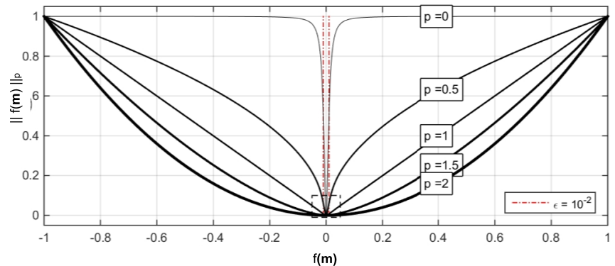
Note that choosing a different \(l_p\)-norm greatly changes how we measure the function \(f(m)\). Rather than simply increasing exponentially with the size of \(f(m)\), small norms increase the penalty on low \(f(m)\) values. As \(p\rightarrow 0\), we attempt to recover as few non-zero elements, which in turn favour sparse solutions.

Since it is a non-linear function with respect to \(\mathbf{m}\), we can linearize it as

\[ \| f(\mathbf{m})_i \|_p \approx \| \mathbf{R}_i \mathbf{W}_i f(\mathbf{m})_i\| \]

where

\[ \mathbf{R}_i = {\frac{1}{\left( {{f(m)^{(k-1)}_i}}^{2} + \epsilon^2 \right)^{1-p/2 }}}\,. \]

Here, the superscript \((k)\) denotes the iteration step of the inversion. This is also known as an iterative re-weighted least-squares (IRLS) method. For more details on the implementation, refer to Fournier and Oldenburg [FO19].

Note on Total Variation

In the literature and other inversion software, sparsity constraints are imposed as an L1-norm on the model gradients, also called Total Variation inversion. While the implementation may differ slightly, the general \(l_p\)-norm methodology presented above encompasses this specific case. We can write

\[ \sum_{i} {|f(m)_i |}^p \approx \sum_{i} {\frac{ (\mathbf{G}_x \mathbf{m})_i^2 + (\mathbf{G}_y \mathbf{m})_i^2 + (\mathbf{G}_z \mathbf{m})_i^2}{\left( (\mathbf{G}_x \mathbf{m})_i^2 + (\mathbf{G}_y \mathbf{m})_i^2 + (\mathbf{G}_z \mathbf{m})_i^2 + \epsilon^2 \right)^{1-p/2 }}} \;. \]

Then for \(p=1\)

\[ \phi(m) \approx \sum_{i} \sqrt{(\mathbf{G}_x \mathbf{m})_i^2 + (\mathbf{G}_y \mathbf{m})_i^2 + (\mathbf{G}_z \mathbf{m})_i^2} \;, \]

which recovers the total-variation (TV) function. Lastly, for \(p=2\)

\[ \phi(m) = \sum_{i} (\mathbf{G}_x \mathbf{m})_i^2 + (\mathbf{G}_y \mathbf{m})_i^2 + (\mathbf{G}_z \mathbf{m})_i^2 \;, \]

which recovers the smooth regularization. The Total Variation (L1) and Smooth (L2) inversion strategies are therefore specific cases of the more general Lp-norm regularization function for \(p \in [0, 2]\).