Interface

Simulating geophysical data from a physical property model requires three things: a computational mesh, a discretization of the model within that mesh, and a means to simulate the data. Plate simulation includes a module for generating a simple two-layer model with embedded plate anomalies within octree meshes. This section discusses all three of these components, their interface exposed by the ui.json file, and the storage of results.

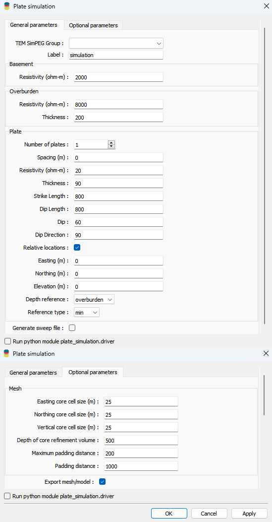
Fig. 51 Merged images of main and advanced parameter tabs.

Forward group

The parameters controlling the forward simulation are defined through a SimPEG forward modelling group. The user must ensure that the SimPEG group has been previously edited with appropriate options, including a topography object, a survey object and data components to simulate.

Oftentimes, the user would like to model a thin plate that might push the resolution limits of the finite-volume approach taken by SimPEG. In this case, the LeroiAir application may be used instead to model the secondary fields from a rectangular prism with a known conductivity-thickness. To use the LeroiAir application for the forward modelling, select the Use LeroiAir checkbox.

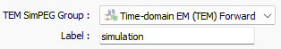
Fig. 52 Selecting the initialized forward modelling SimPEG group, or optionally choosing LeroiAir for improved thin plate modelling and providing a name for the results group.

• Create the required SimPEG group within Geoscience ANALYST through the Geophysics menu under SimPEG Python Interface entry.

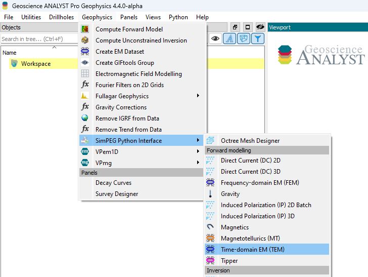
Fig. 53 Creating a SimPEG group to be selected within the plate simulation interface.

• Edit the options by right-clicking the group and selecting Edit Options.

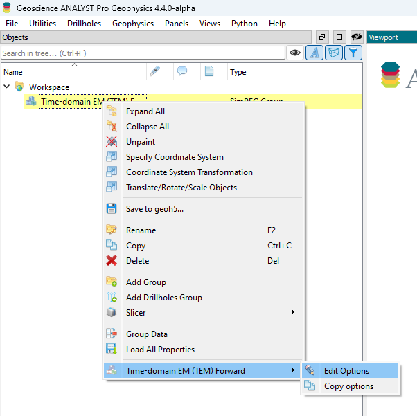
Fig. 54 Editing the SimPEG group options.

Since plate-simulation creates its own mesh and model, the mesh and conductivity selections can be ignored. Selecting a value does not conflict with the plate-simulation objects and is simply ignored.

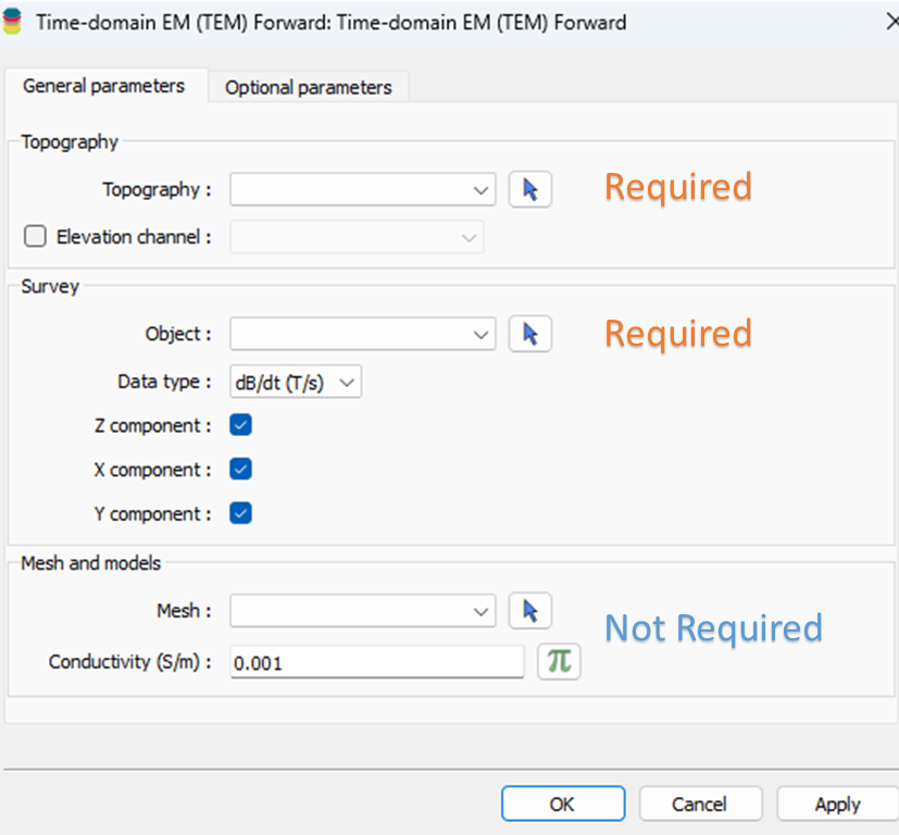
Fig. 55 Simulation options with annotations for required and not required components.

Label

The user may also provide a name for the new SimPEG group to store the results.

Geological Model

Plate simulation includes a module for generating plates embedded in a two-layer Earth model within octree meshes. Many permutations of this simple geological scenario result in a complex interface. To simplify this, the discussion is organized into two subsections: background (basement and overburden) and plates. All model values within plate-simulation must be provided in SI units that varies depending on the chosen forward simulation (g/cc, SI or Ohm.m)

Basement

The basement physical property fills the model below the overburden layer.

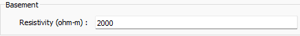
Fig. 56 Basement physical property option.

Overburden

The overburden is discretized by a physical property value and a thickness.

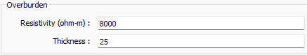
Fig. 57 Overburden physical property and thickness options.

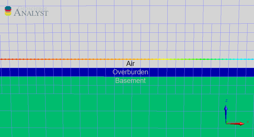
Fig. 58 Model section highlighting the overburden and basement boundary.

Plates

This section discusses the various options to define the plate(s) embedded in the basement, below the overburden layer.

Users can specify the number of plates and the spacing between them.

Fig. 59 Number of plates and spacing options.

For all choices of n>1, the plates are evenly spaced at the requested spacing. All plates share the same physical property, size, and orientation.

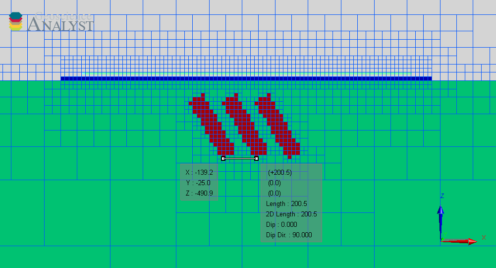
Fig. 60 Model created by choosing three plates spaced at 200m.

The plate physical property must be entered in SI units (g/cc, SI or Ohm.m).

The size of the plate is defined by three parameters: thickness, strike length, and dip length.

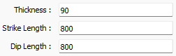
The image below shows a dipping plate with annotations indicating the size parameters for that particular plate.

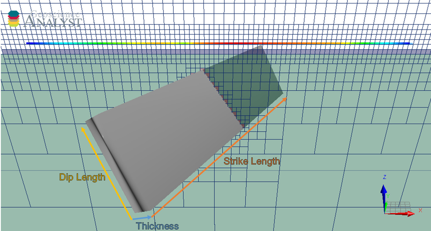
Fig. 61 A dipping plate striking northeast with annotations for its thickness, strike length and dip length.

The plate orientation is defined in terms of dip and dip direction. The dip is the angle between the horizontal projection of the plate normal and the plate tangent sharing the same origin. The dip direction is measured between the horizontal projection of the plate normal and the North arrow. The image below provides a visual representation of these angles.

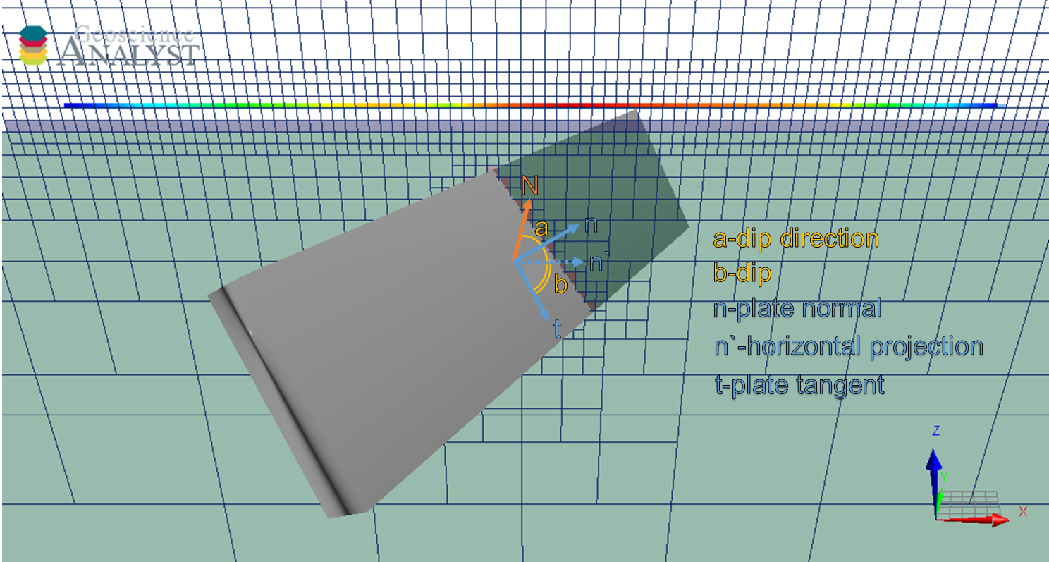
Fig. 62 Plate orientation options. Plate orientation is given as a dip and dip direction. The dip (b) is defined as the angle between the horizontal the projection of the plate normal (n’) and the plate tangent sharing the same origin (t). The dip direction (a) is the angle measured between the horizontal projection of the plate normal (n’) and due north (N).

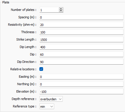
The plate location is chosen to be centered on the provided survey object with the depth relative to the topography entered as positive down.

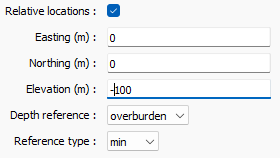
Fig. 63 Plate depth option sets the top of the plate n meters below the topography and centered on the survey object.

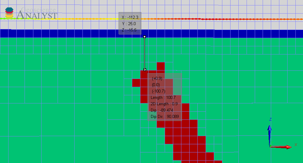
Fig. 64 Example of a relative elevation referenced 100m below the minimum of the overburden layer.

Octree Mesh

To accurately simulate the earth model, the mesh must be refined in key areas while remaining coarse enough elsewhere to efficiently simulate data. Plate simulation includes refinements at the earth-air interface, the transmitter and receiver sites, and on the surface of plates.

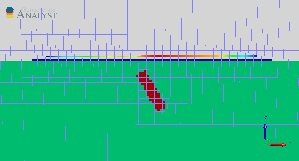
Fig. 65 Octree mesh refinement for earth-air interface, receiver sites, and within the mesh.

The meshing is controlled by options exposed in the ui.json. These options are significantly reduced compared with octree creation from grid-app, as many parameters have been tailored to suit the needs of plate simulation.

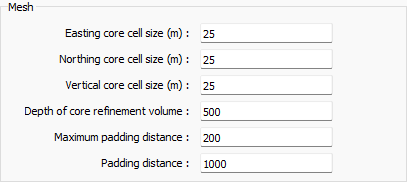
Fig. 66 Octree mesh parameters exposed in the ui.json file.

Results

The results of the simulation are stored in the SimPEG group named in the Forward group section.

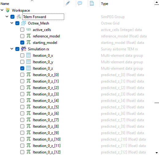
Fig. 67 Results group containing a survey object with all the simulated data channels stored in property groups, and an octree mesh containing the model parameterized in the interface.

To iterate on the design of experiment, copy the options, edit them, and run again.

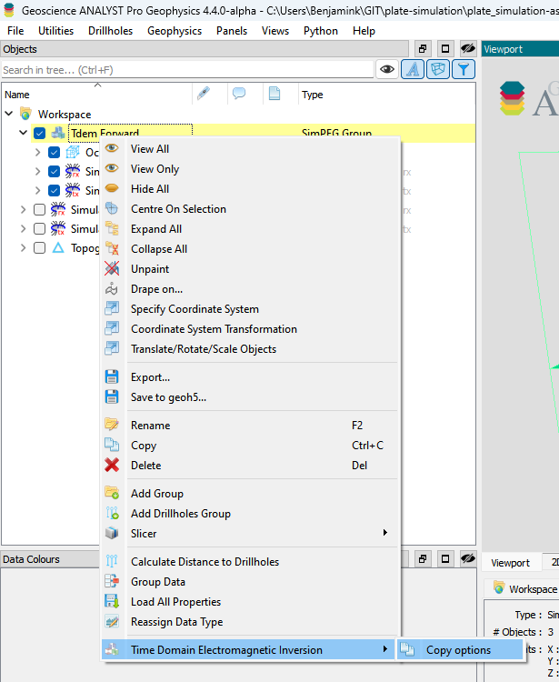
Fig. 68 Copying the options to run a new simulation.