
Airborne Time-Domain EM (ATEM) Inversion#
This section focuses on the inversion of airborne time-domain data generated from the Flin Flon conductivity model.
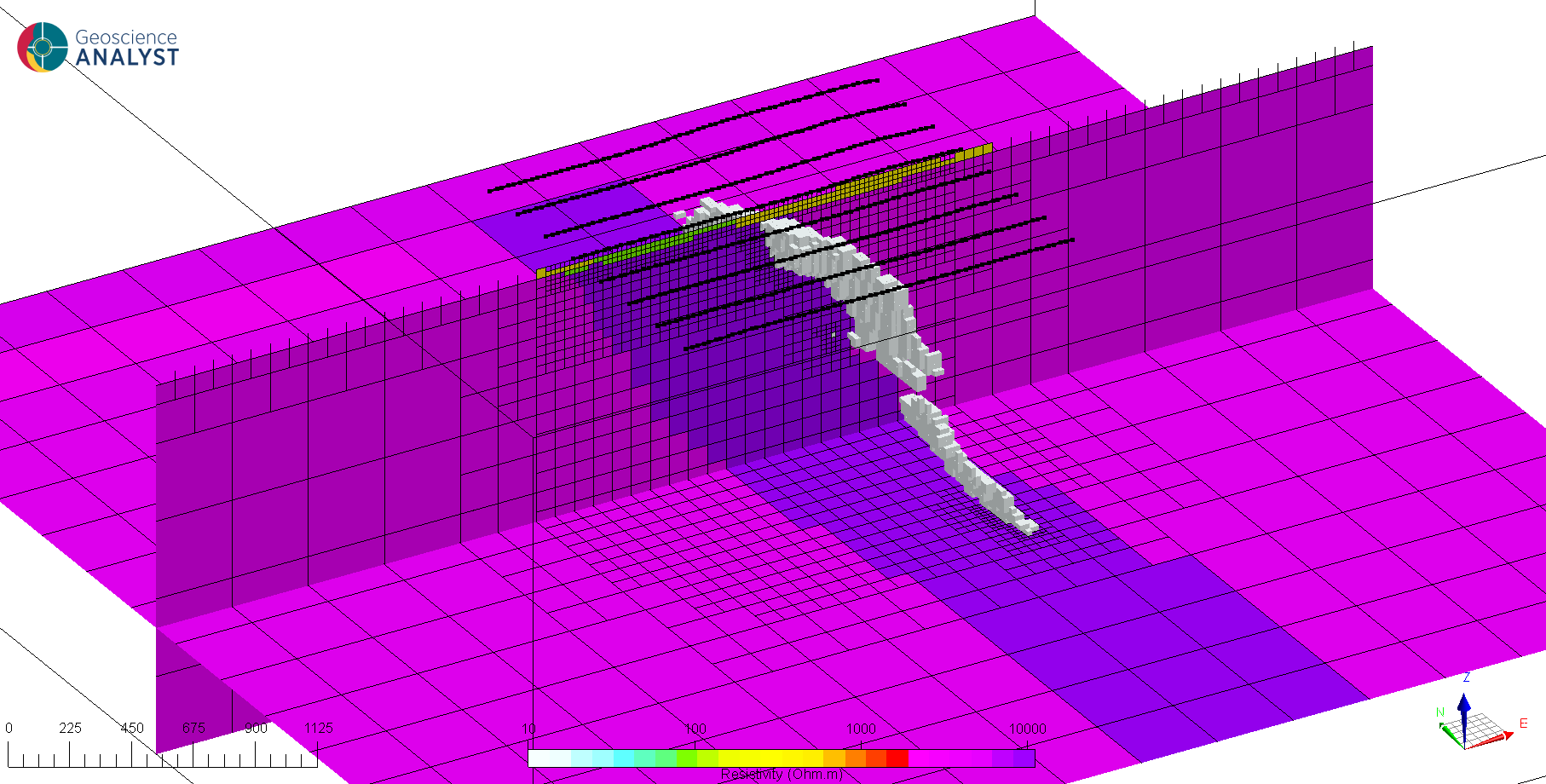
Fig. 29 Download here#
Note
Runtime and memory usage increases rapidly with the mesh size and number of sources. It is strongly recommended to downsize this example to a few lines if the training is done on a standard computer. The full inversion presented below was performed on an Azure HC44rs node (44 CPUs, 315 Gb RAM) in ~2.0 h.
ATEM data#
Time-domain systems come in many configurations, but they are generally made up of
an horizontal transmitter loop
a receiver coil.
The transmitter emits an EM pulse that propagates and interacts with conductive structures. During the off-time, the receiver(s) records either components of the magnetic field (\(H_x,\;H_y,\;H_z\)), or more commonly the time-derivative (\(\frac{\delta B_z}{\delta t}\)) of the field over a range of time channels. For more background information about airborne EM methods, see em.geosci
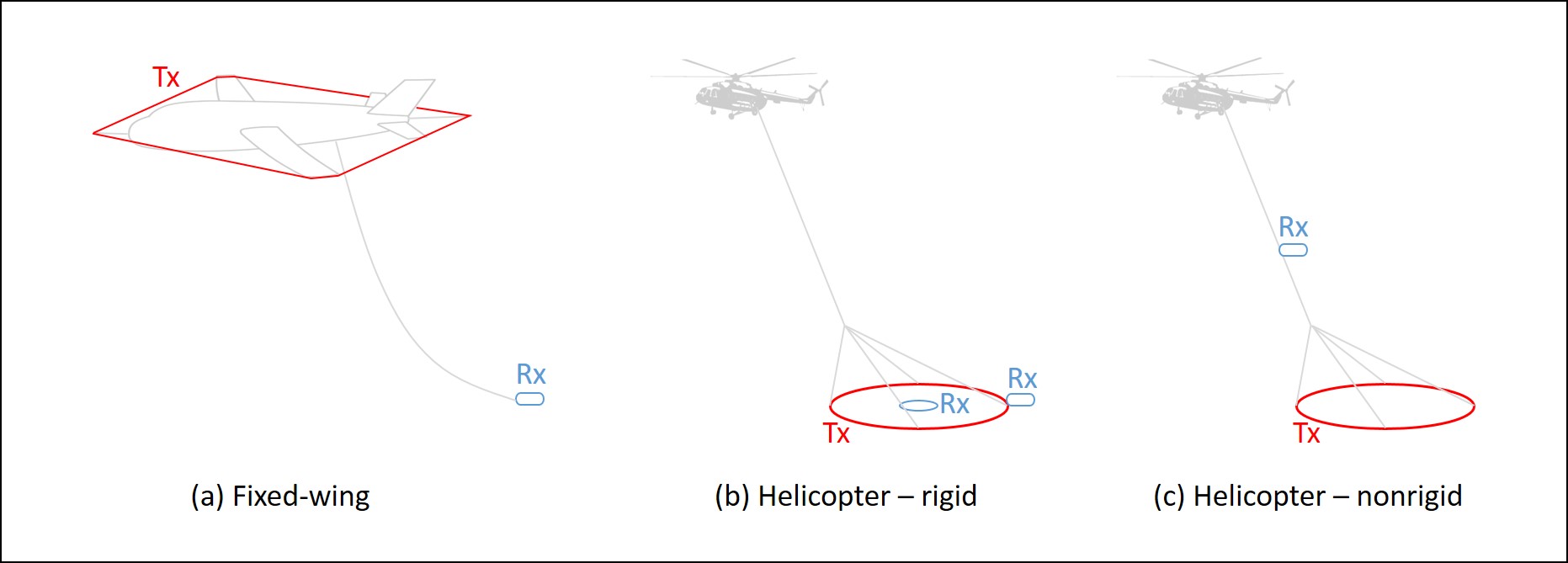
Fig. 30 Various ATEM source-receiver configurations. Borrowed from em.geosci.#
For this tutorial, we generated an airborne time-domain EM survey over the main ore body. The survey lines are spaced at 400 m, oriented East-West, at a drape height of 60 m. The configuration used in this tutorial is a simplified version of typical airborne systems, with only five time channels measuring \(\frac{\delta B_z}{\delta t}\) between 1 to 10 milli-seconds.
Waveform#
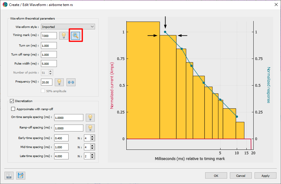
In order to properly model the EM fields, it is necessary to specify the EM source - commonly known as the waveform. Most contractors will provide an ASCII file containing times and currents describing the waveform, which can be loaded directly in ANALYST (Download example). For the purpose of this tutorial we are using a simple theoretical trapezoidal function.
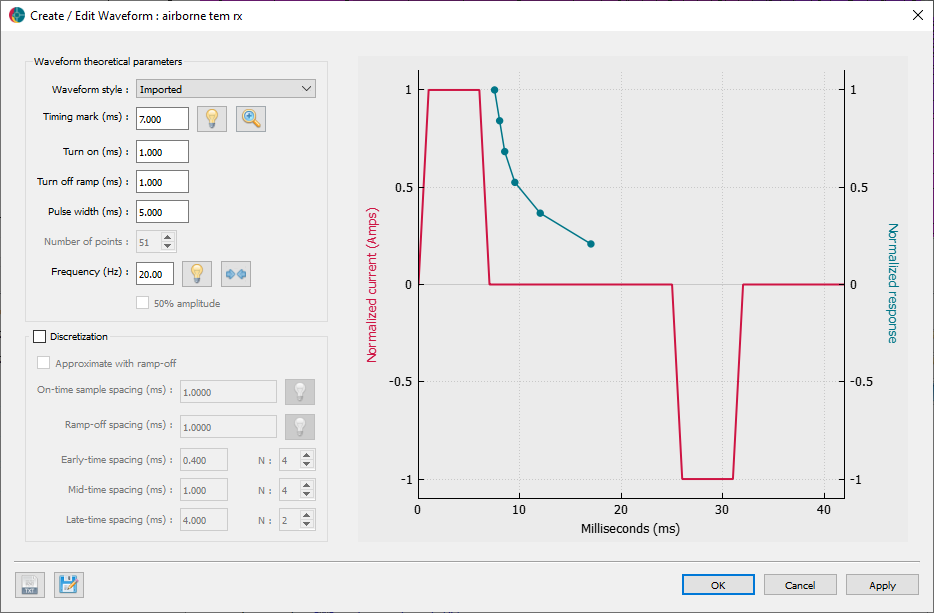
Fig. 31 (red) Trapezoidal waveform with 5 msec pulse with, 20 Hz duty cycle and (blue) time channels recording data during the off-time.#
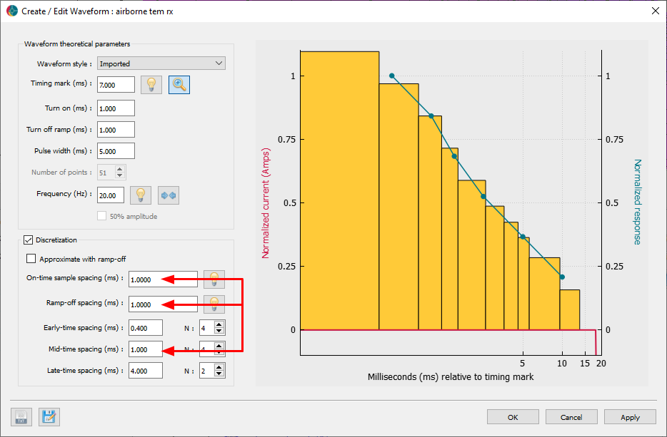
As part of the numerical simulation, this waveform must be discretized. That is, the theoretical waveform must be sampled at discrete time intervals. The forward simulation uses those steps to simulate the EM field over time. A few important details must be taken into account to preserve good numerical accuracy while optimizing runtime and memory usage:
Discrete intervals must cover the entire wave cycle, from start of the pulse to past the last recording.
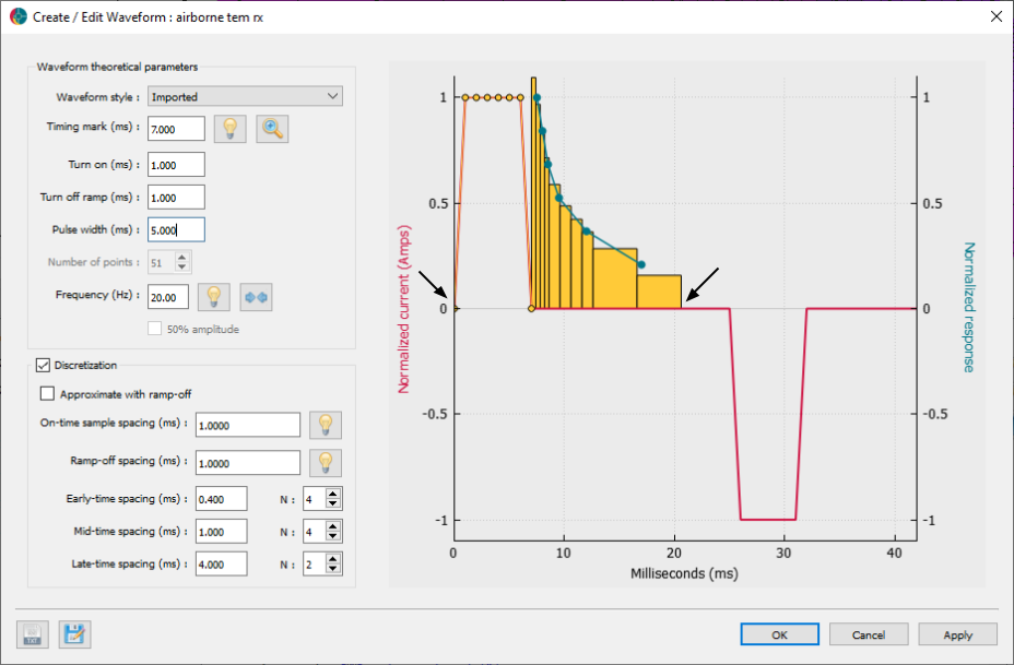
Time steps should only contain at most one time channel
Optimization
Minimizing the total number of time steps will speed up the the forward simulation.
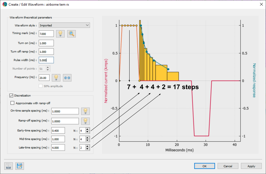
The direct solver used by the forward simulation requires a matrix factorization for each unique time step width. Whenever possible, reuse time step intervals to reduce memory requirements.
Mesh creation#
In preparation for the inversion, we create an octree mesh optimized for the airborne TEM survey. The mesh parameters are base on the original Flin Flon model.
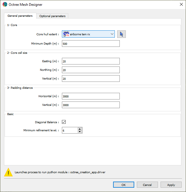
Fig. 32 Core mesh parameters.#
Note that the padding distances are set substantially further than for the magnetics, gravity or dc-resistivity (1 km) inversions. This is because the diffusion distance for a background resistivity of \(1000 \; \Omega .m\) for the last time channel (10 msec) is roughly 3.3 km. This distance is important to satisfy the boundary conditions of the underlying differential equations.
Refinements#
For the first refinement, we insert 4 cells for the first three octree levels along the flight path. The refinement is done radially around the segments of the flight path curve to assure good numerical accuracy near the receiver locations. This is especially important for EM methods with low frequencies.
We use a second refinement along topography to get a coarse but continuous air-ground interface outside the area or interest.
Lastly, we refine a “horizon” to get a core region at depth with increasing cell size directly below the survey. This is our volume of interest most strongly influenced by the data.
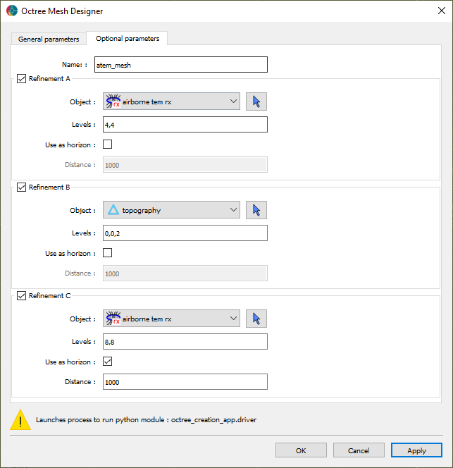
Fig. 33 Refinement strategy used for the atem modeling.#
See Mesh creation section for general details on the parameters.
Forward simulation#
Having defined the TEM survey, we can proceed with the forward simulation using the conductivity Flin Flon model.
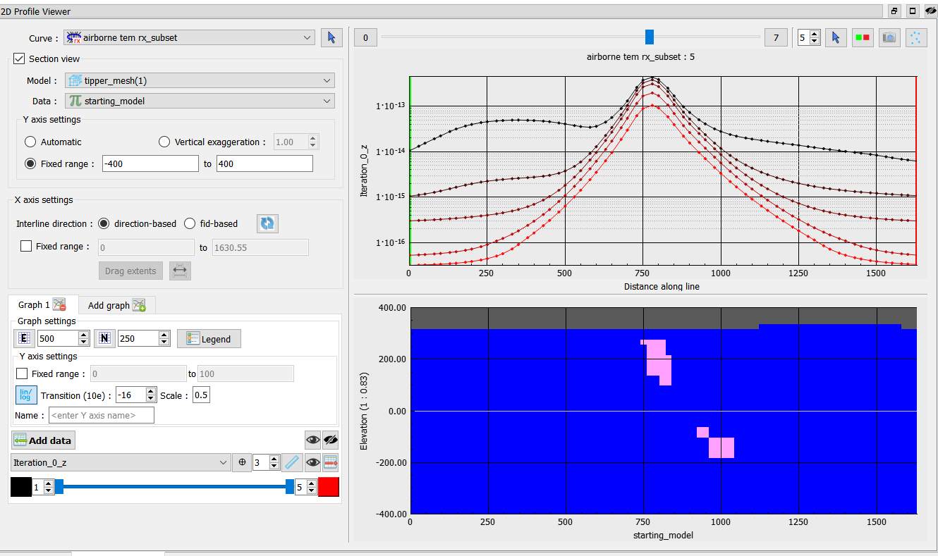
Fig. 34 (Top) ATEM \(\frac{\delta B_z}{\delta t}\) data displayed by the 2D Profiler at all 5 time channels. (Bottom) Survey lines relative to (left) the ore body and (right) the discrete conductivity model.#
Note that the position of the known conductor correlates with large amplitude in the ATEM data .
Unconstrained inversion#
Runtime: ~2.0 h
Time-domain EM data involves data measured over a wide range of time channels that decays over several orders of magnitude. Balancing all this data can be challenging and time consuming. Here we adopt a percentage and floor uncertainty strategy.
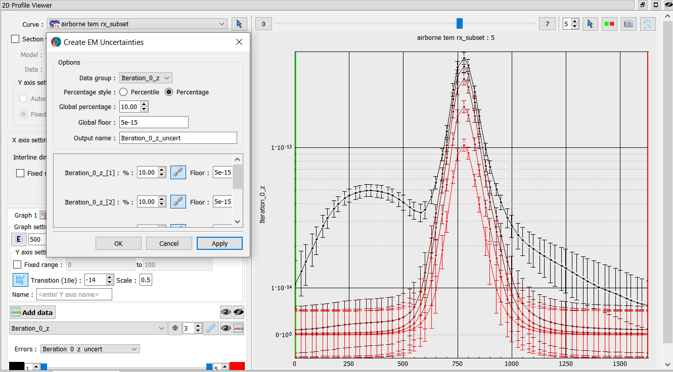
This approach is a good starting point, but experimentation is generally required.
After running the inversion we recover the following solution:
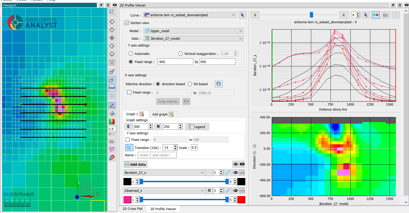
Fig. 35 (Left) Horizontal section at 120 m elevation after reaching target misfit (iteration 5).#
(Right)(top) 2D profiles of (red) observed versus (black) predicted data for all 5 time channels. (bottom) Vertical section through the conductivity model below the same line.
Despite our simplistic floor uncertainties, the inversion managed to converge fairly quickly to a reasonable model that fits our data well. We have recovered a clear conductor at depth that overlaps with the ore body. The inversion could resolve the conductive overburden layer, although the thickness is overestimated.