
Gravity Inversion#
This section focuses on the inversion of airborne tensor and ground gravity data generated from the Flin Flon density model.
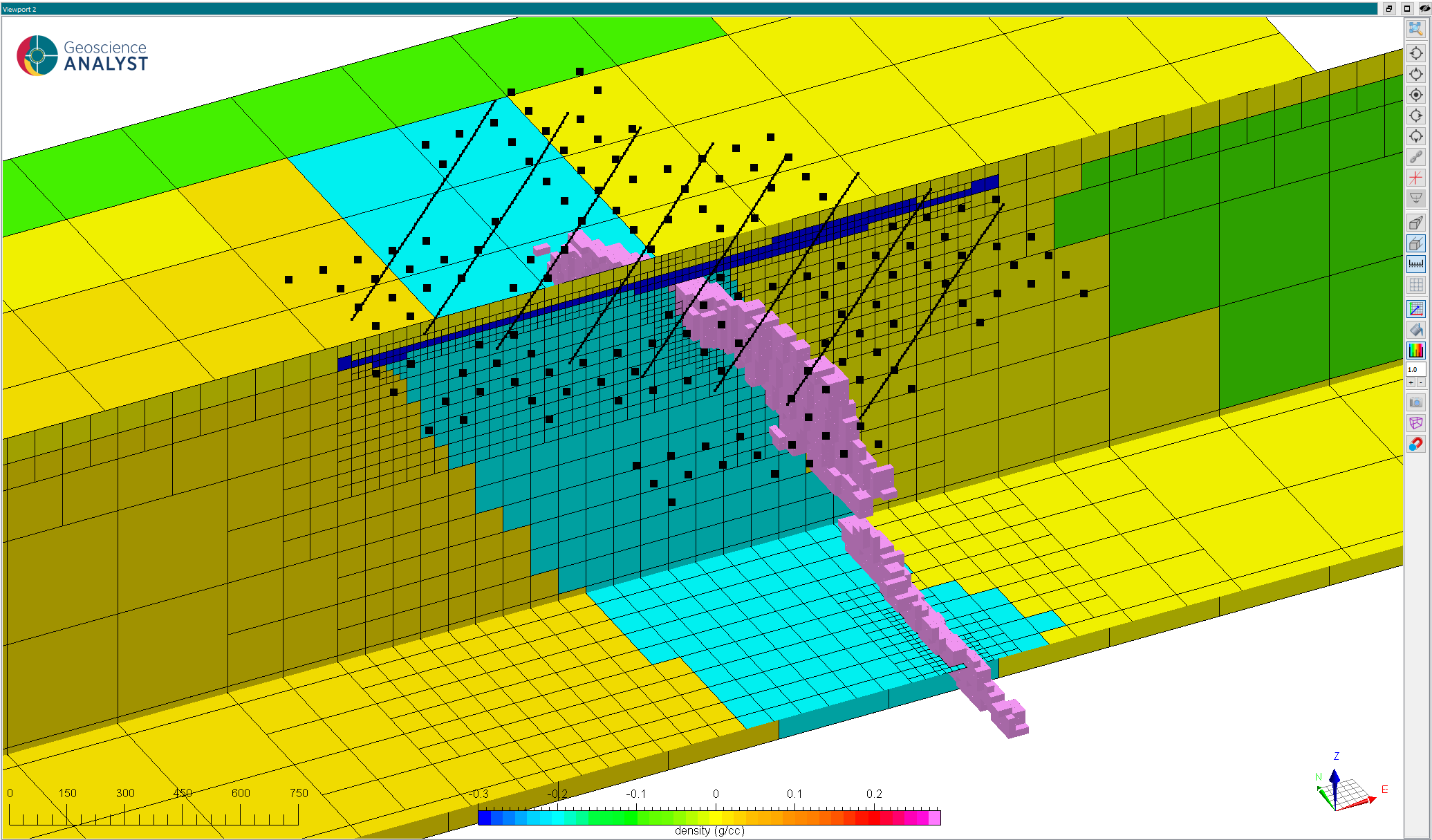
Fig. 12 Download here#
Forward simulation#
A ground gravity survey was simulated on sparsely sampled 200 m grid of stations.
The following parameters were used for the forward simulation:
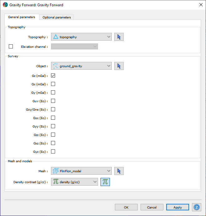
After running the forward simulation, we obtain gravity corrected data as shown below. The gravity survey appears to be mostly influenced by the large formations, with little signal apparent from the ore body. Since we have used relative densities, the simulated data is equivalent to a terrain correction with reference density, of 2.67 g/cc in this case.

Fig. 13 Vertical component of the gravity field (gz) measured over the zone of interest.#
Mesh creation#
In preparation for the inversion, we create an octree mesh optimized for the gravity survey.
The core param are as follow:
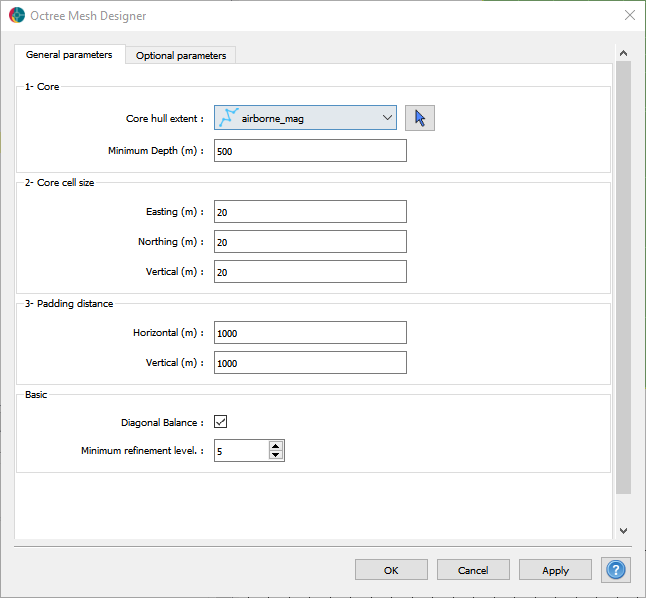
Fig. 14 Core mesh parameters.#
Refinements#
The first refinement “horizon” is used to get a core region at depth with increasing cell size directly below the survey. This is our volume of interest most strongly influence by the data. We use a maximum distance of 100 m to limit the refinement near each station.
A second refinement is used along topography to get a coarse but continuous air-ground interface outside the area or interest.
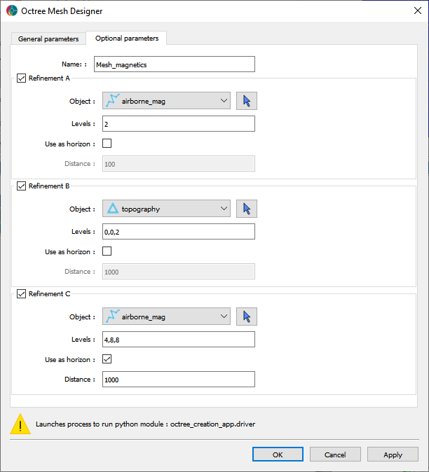
Fig. 15 Refinement strategy used for the magnetic modeling.#
See Mesh creation section for general details on the parameters.
Ground gravity#
The ground gravity data are assigned a constant floor uncertainty value of 0.1 mGal. We apply the the following inversion parameters:
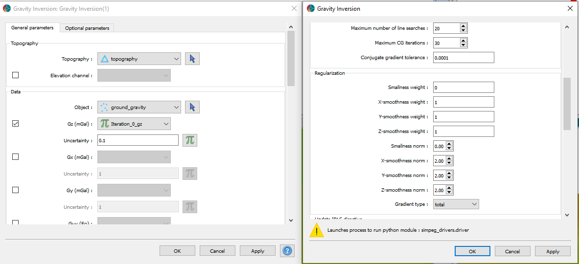
After running the inversion we obtain:
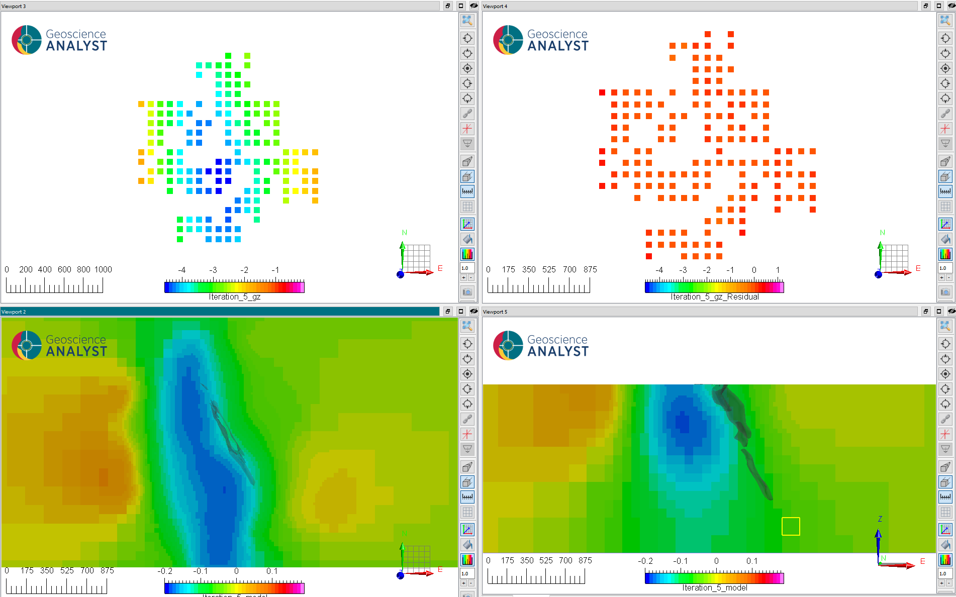
Fig. 16 (Top) (left) Predicted and (right) residuals data after reaching target misfit (iteration 5).#
(Bottom) Slices through the recovered relative density model: (left) at 175 m elevation and (right) at 6072150 m N. Ore shell is shown for reference.
Notice that the inversion resolves the boundaries between the rhyolite unit and host mafic units, but poorly recovers the ore body. That is, the ore body does not generate a gravity anomaly strong enough within the host geology to be detected by the ground gravity survey.
Tensor gravity gradiometry (FTG)#
We now look at the airborne fixed-wing full-tensor gravity gradiometry (FTG) data. The FTG system measures six independent components of the gradient tensor: \(g_{xx},\; g_{xy},\; g_{xz},\; g_{yy},\; g_{yz}\) and \(g_{zz}\). We generate a survey flown at 45 degree azimuth, 200 m line spacing, at a nominal drape height of 60 m above topography.
Using the same relative density model as previously, we run the forward simulation and obtain terrain-corrected data show below.
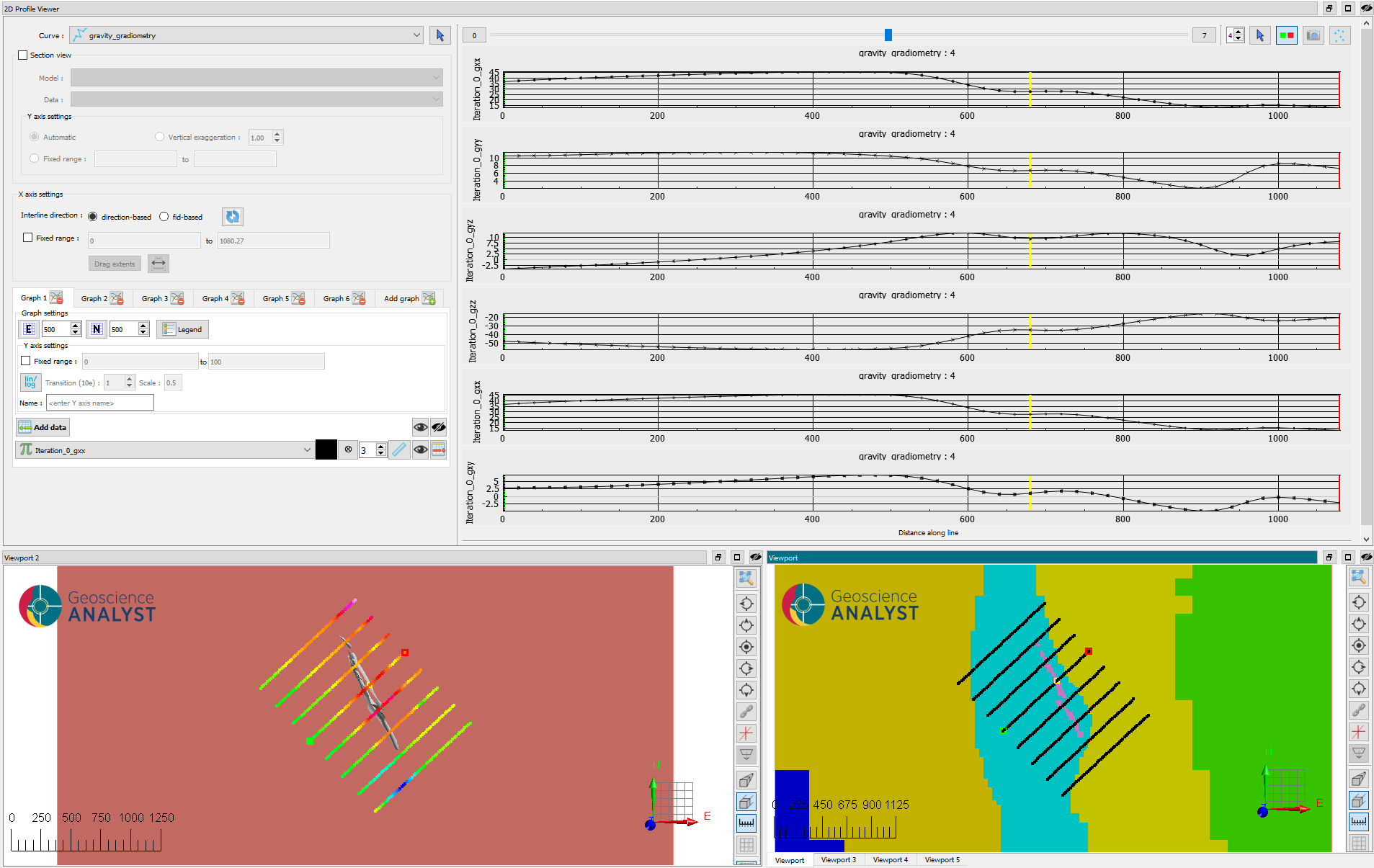
Fig. 17 (Top) Components of the gravity gradiometry data measured over the zone of interest. (Bottom) Plan view of the density model and flight lines. The green and red marker indicate the flight direction.#
Unconstrained FTG#
We repeat the same inverse process as for the ground gravity data, but this time with the airborne survey. A floor uncertainty value of 0.1 Eotvos was assigned to all the components. After running the inversion with obtain.
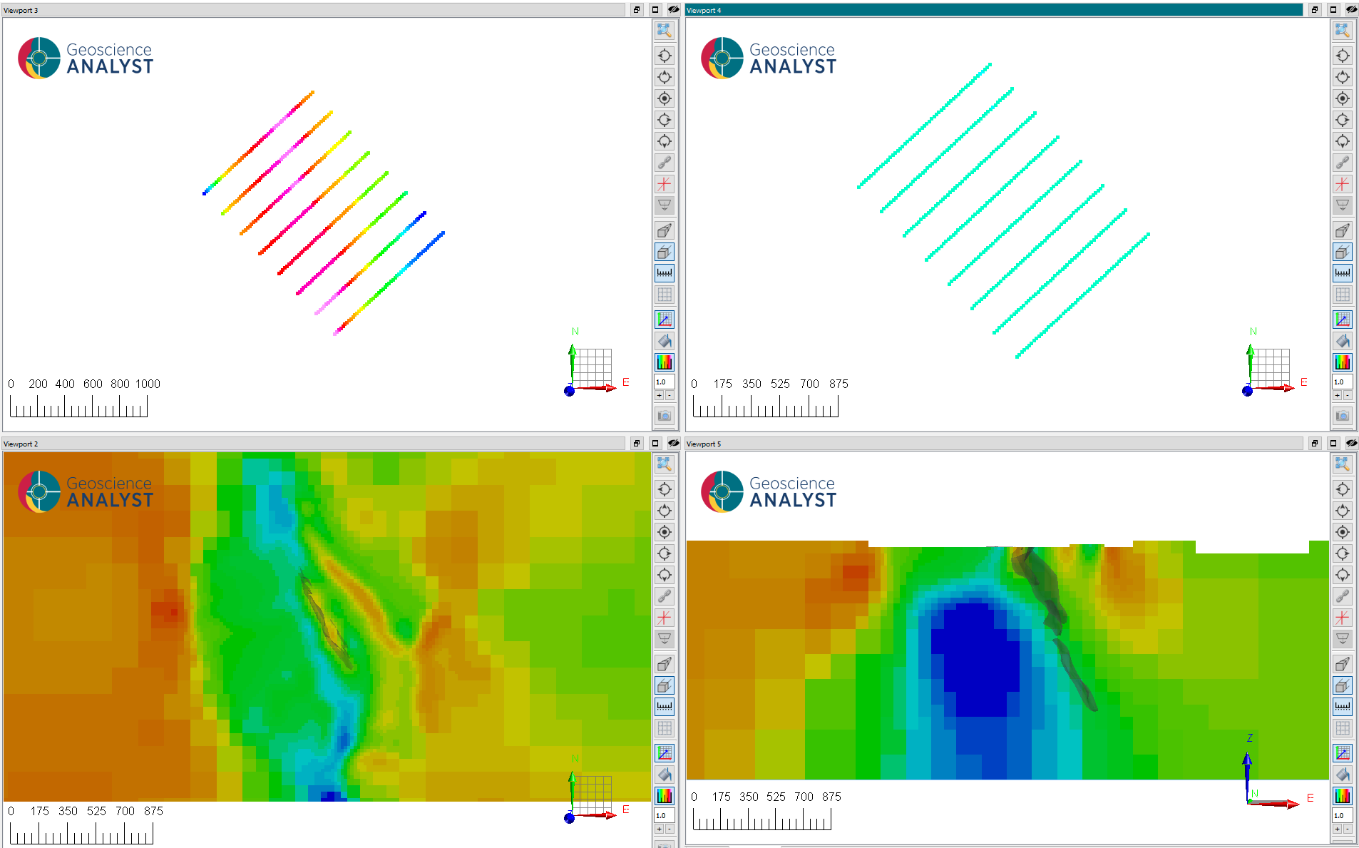
Fig. 18 (Top) (left) Predicted and (right) residuals data after reaching target misfit (iteration 7).#
(Bottom) Slices through the recovered relative density model: (left) at 175 m elevation and (right) at 6072150 m N. Ore shell is shown for reference.
Just like the ground gravity result, the airborne inversion recovers well the boundary between the rhyolite and host mafic rocks. The ore body is also imaged on the top 200 m. In addition, we recover density structures within the Hidden Formation related to the overburden layer.
Detrending#
Section to explain different strategies for regional signal removal
Polynomial
Scooping method