
Magnetic Inversion#
This section focuses on the inversion of magnetic data using a scalar (susceptibility) and a magnetization (vector) approach generated from the Flin Flon magnetic model. We also cover some strategies on how to remove regional signal and the use of compact norms.
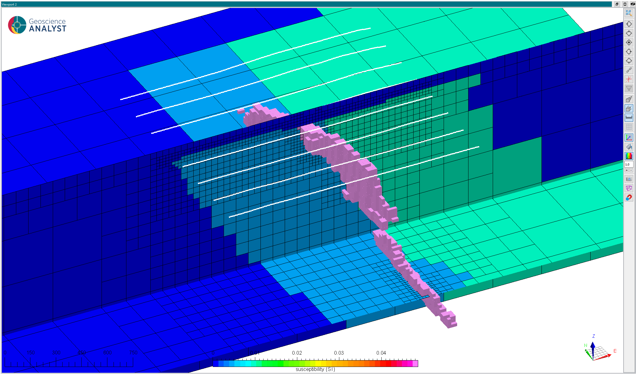
Fig. 5 Download here#
Forward simulation#
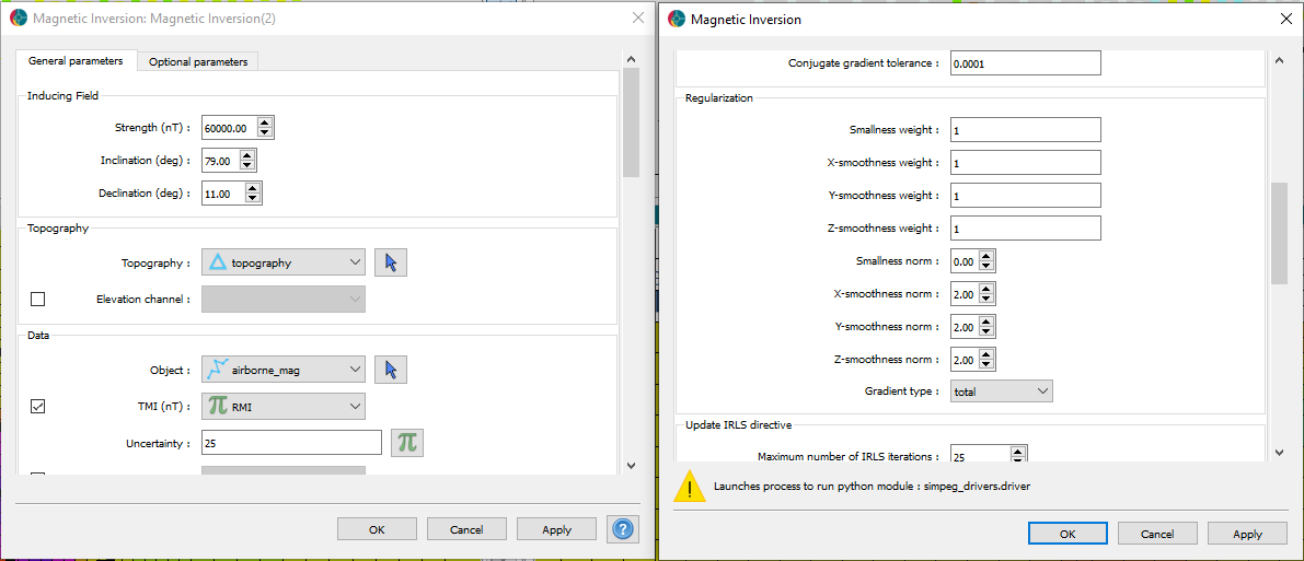
We simulated Residual Magnetic Intensity (RMI) data along East-West lines spaced to 200 m apart, with along-line data downsampled to 10 m. The flight height is set to 40 m above topography.
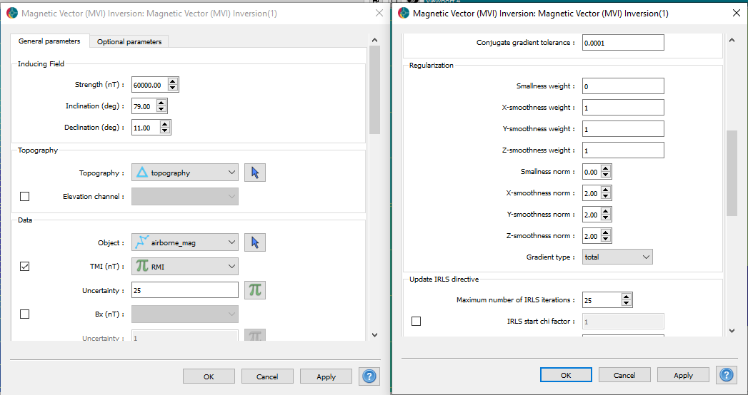
The following parameters were used for the forward simulation:
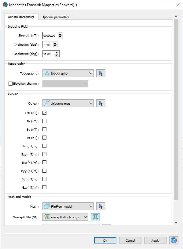
For simplicity, the simulation assumes a purely induced response. By omitting to supply values/models for the inclination and declination of magnetization, the forward routine uses the inducing field parameters instead.
After running the forward simulation, we obtain RMI data as shown below. We note the strong correlation between the amplitude of the signal and the horizontal position of the ore body. There is also a significant long wavelength East-West trend, due to the large but weakly magnetic Hidden Formation.
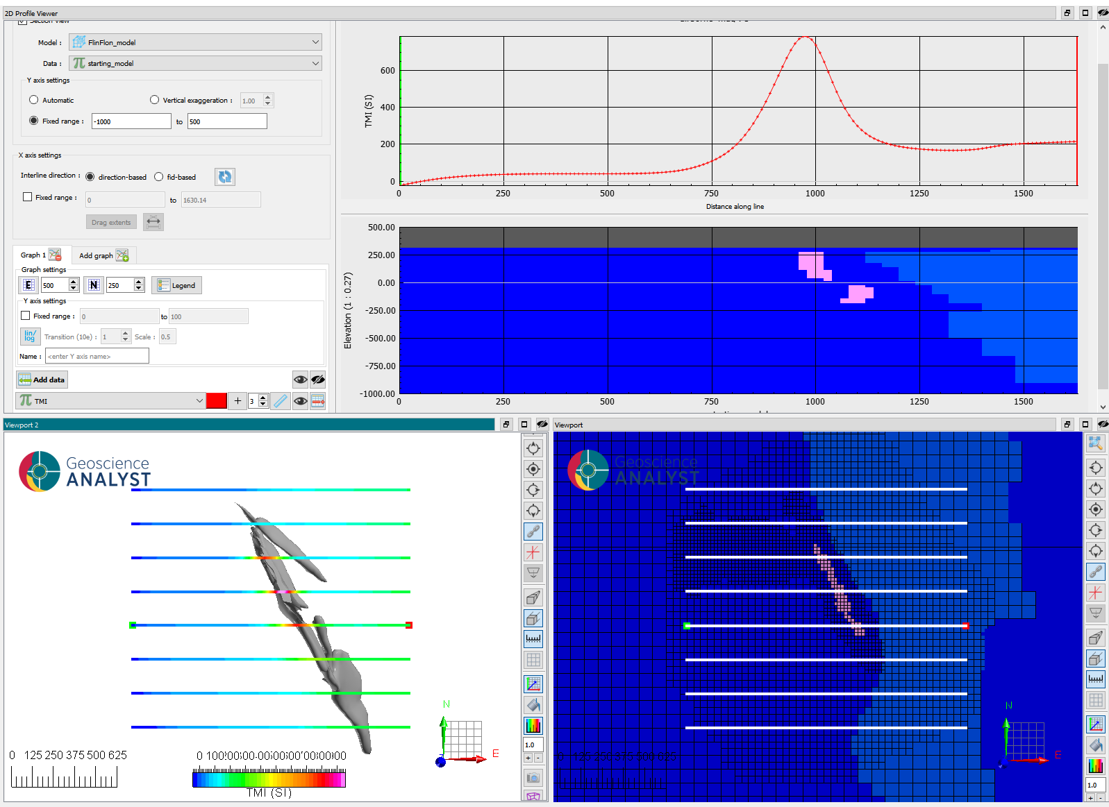
Fig. 6 Residual magnetic intensity (RMI) data measured over the zone of interest.#
Mesh creation#
In preparation for the inversion, we create an octree mesh optimized for the magnetic survey. The following parameters are used based on the original Flin Flon model.
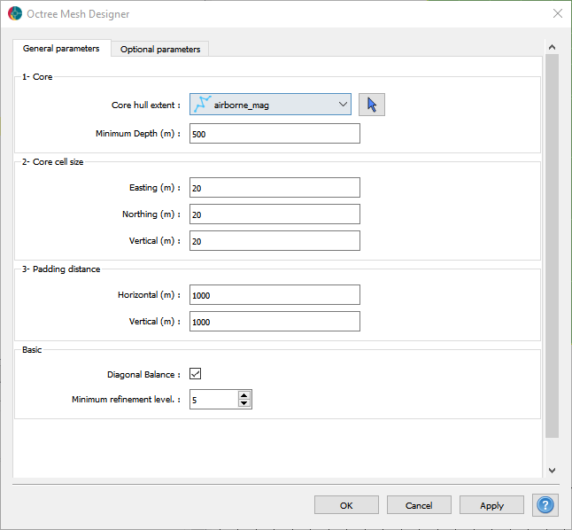
Fig. 7 Core mesh parameters.#
Refinements#
For the first refinement, we insert two cells around our survey lines. The refinement is done radially around the segments of the curve to assure that the air-ground interface near the receivers are modeled with the finest cell size.
A second refinement is used along topography to get a coarse but continuous air-ground interface outside the area or interest.
The third refinement “horizon” is used to get a core region at depth with increasing cell size directly below the survey. This is our volume of interest most strongly influence by the data.
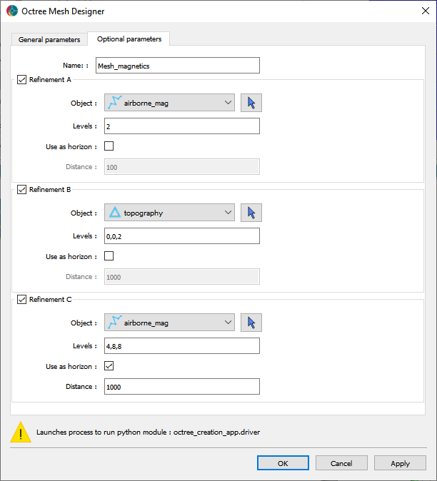
Fig. 8 Refinement strategy used for the magnetic modeling.#
See Mesh creation section for general details on the parameters.
Scalar inversion (susceptibility)#
Runtime: ~1 min
As a first pass, we invert the data with default parameters. We use a constant 25 nT floor uncertainty, determined empirically to achieve good fit.
After running the inversion we obtain:
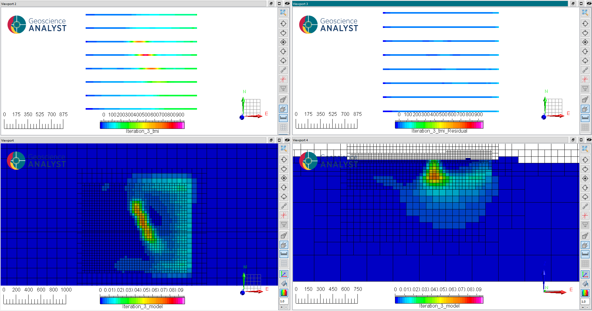
Fig. 9 (Top) (left) Predicted and (right) residuals data after reaching target misfit (iteration 3).#
(Bottom) Slices through the recovered susceptibility model: (left) at 175 m elevation and (right) at 6072150 m N.
We note that our model predicts the data within our uncertainty floor of 25 nT. In plan view, the model shows a clear North-West trend corresponding to the ore body. On the vertical section we recover an isolate body at depth. We note that large portions of the model in the padding cells have no anomalies. All the magnetic signal is confined to a region directly below the survey lines.
This is somewhat surprising given the large East-West trend in the data, which would be better explain by a large body extending beyond the extent of our survey. Let’s confirm this solution with a second inversion.
No reference model#
As a second pass, we test whether our initial assumption of a uniform zero susceptibility model is adequate. We can remove the influence on the reference model by setting the corresponding scaling factor to 0. After re-running the inversion we recover:
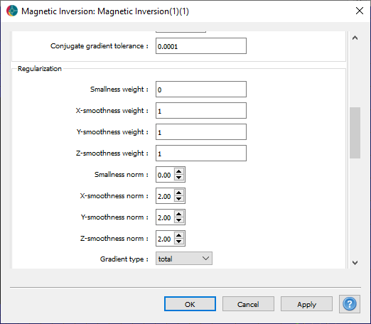
The model shown below generally agrees with the position of the strongly magnetic ore body, but changes greatly outside the survey area. Since we have not imposed any constraints on the background value, the inversion is free to extend the smoothout the eastern anomaly both at depth and in the padding region. This is in better agreement with our known geological knowledge.
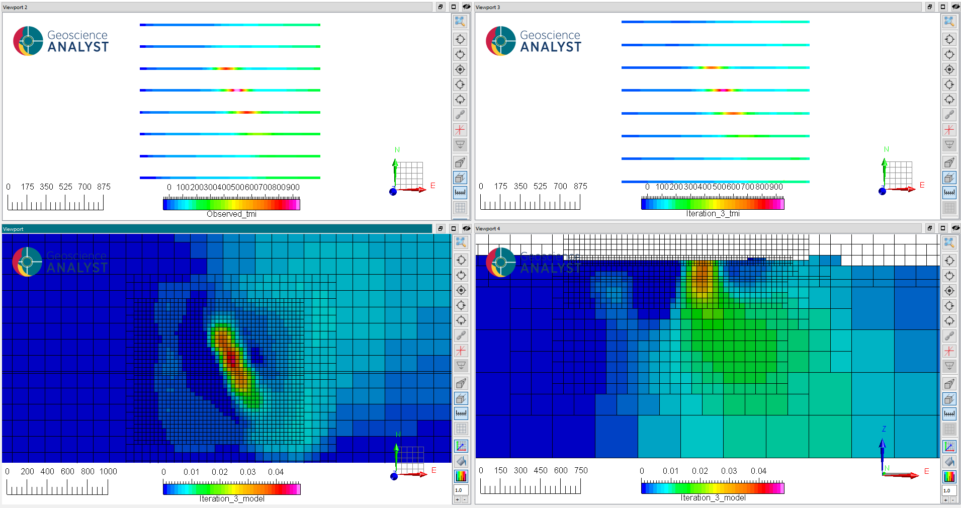
Fig. 10 (Top) (left) Predicted and (right) residuals data after reaching target misfit (iteration 3).#
(Bottom) Slices through the recovered susceptibility model: (left) at 175 m elevation and (right) at 6072150 m N.
Magnetic vector inversion (MVI)#
We now look at the solution using the magnetic vector inversion (MVI) algorithm. This approach is generally favoured if remanent magnetization is kwown to distorte the magnetic signal.
We use the default parameters but without a reference model as shown below.
After running the inversion, we obtain
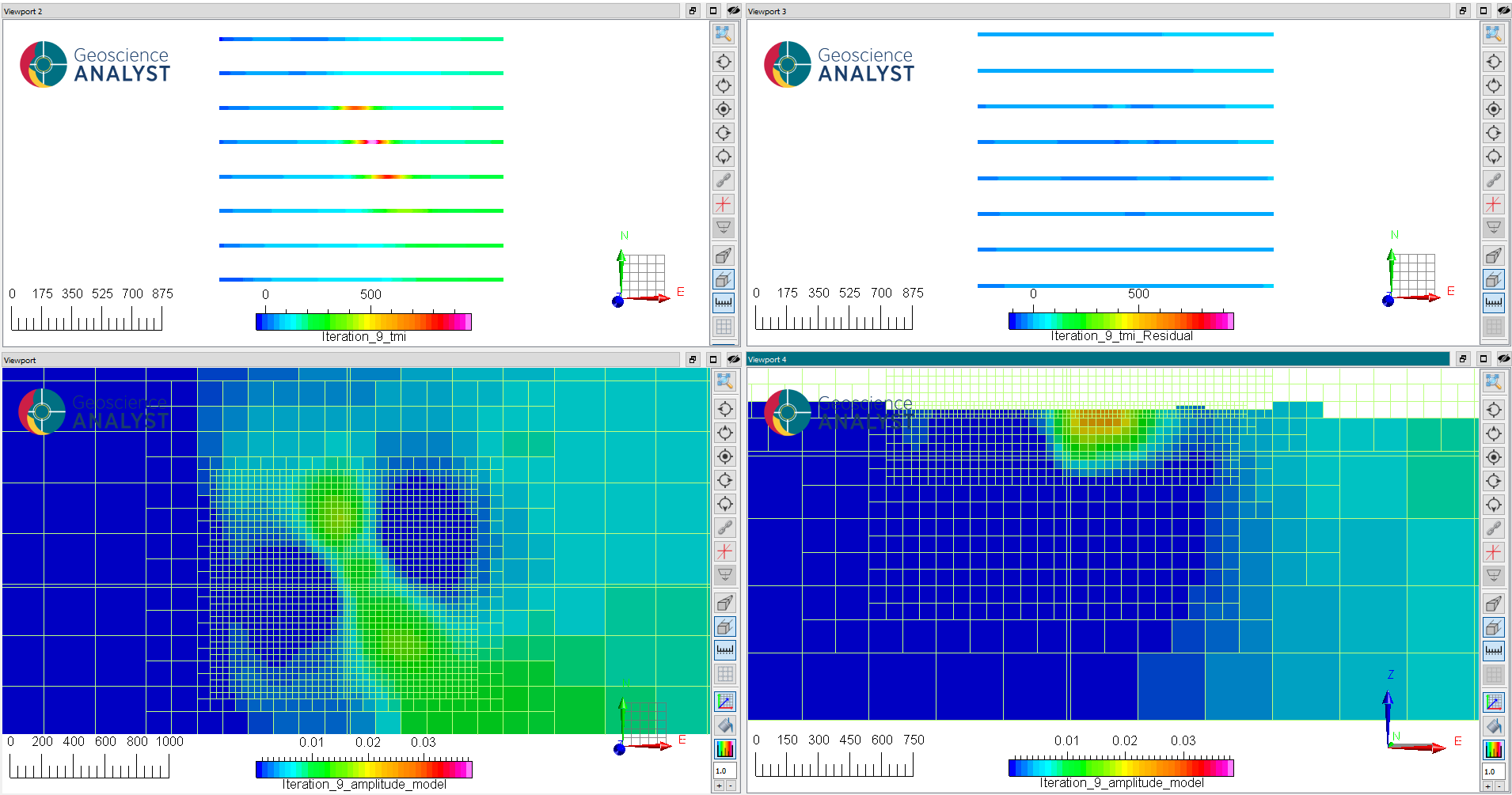
Fig. 11 (Top) (left) Predicted and (right) residuals data after reaching target misfit (iteration 3).#
(Bottom) Slices through the recovered susceptibility model: (left) at 175 m elevation and (right) at 6072150 m N.
We note that the effective susceptibility values are much lower than recovered with the scalar susceptibility inversion. The anomaly is also smoother, broader and less well defined at depth. This can be explained by the increase in non-uniquess of the inverse problem, where we now have to solve for three models (vectors) at once. This result could be improved with additional constraints, but beyond the scopy of this section.
Algorithmic details#
Looking back at the log file, users may notive that the MVI process goes through three main stages:
1- Solve the problem in Cartesian (3-components) form for a smooth model
2- Convert the model to Spherical (amplitude and angles) and iterate to target misfit.
3- Use the smooth Spherical model for the compact IRLS iterations.
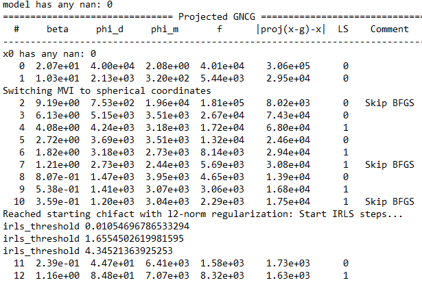
Note that the last Cartesian model ends after reaching a target misfit of about 2x (hard-coded). User should preferentially use the last model from the Spherical steps, or last of IRLS, to do their interpration as both are on or near target.
See Fournier et al. 2020 for more details.