Data Fitting

The data misfit function (\(\phi_d\)) measures the quality of a model \(\mathbf{m}\) at fitting the observed data. It generally takes the form

\[ \phi_d =\sum_{i=1}^{N}\left(\frac{d_i^{pred} - {d}_i^{obs}}{w_i}\right)^2 \;. \]

It measures the sum of weighted residual between observed (\(\mathbf{d}^{obs}\)) and predicted (\(\mathbf{d}^{pred}\)) data. In matrix form, this least-square measure can be written as

\[ \phi_d =(F(\mathbf{m}) - \mathbf{d}^{obs})^T \mathbf{W}_d^T \mathbf{W}_d (F(\mathbf{m}) - \mathbf{d}^{obs})\;, \]

where \(F(\mathbf{m})\) is a forward simulation of data (gravity, magnetic, EM, etc.) due to a model \(m\). The \(\mathbf{W}_d\) is a diagonal matrix holding the data weights (\(\frac{1}{\mathbf{w}}\)), also referred to as data uncertainties. The larger the weights, the less importance a given datum has on the solution. There are many sources of noise that can yield large data residuals:

• Experimental noise from \(\mathbf{d}^{obs}\), generally introduced during acquisition (positioning, instrumental noise)

• Numerical noise introduced by \(F(\mathbf{m})\) from our inability to perfectly simulate the physics (discretization, interpolation, etc.)

In all cases, we may never expect the data residual to completely vanish, but we may allow it to be within an acceptable level of fitness for modelling purposes.

Uncertainties

As mentioned in the Data Misfit section, we want to assign data uncertainties that reflect our inability to perfectly replicate the observed data, within an acceptable level. While many strategies can be used, we are going to demonstrate basic principles to assess the effectiveness of a chosen method. We will employ two basic strategies:

• Floor value set as a constant,

• Amplitude-based (%) values with variable weights.

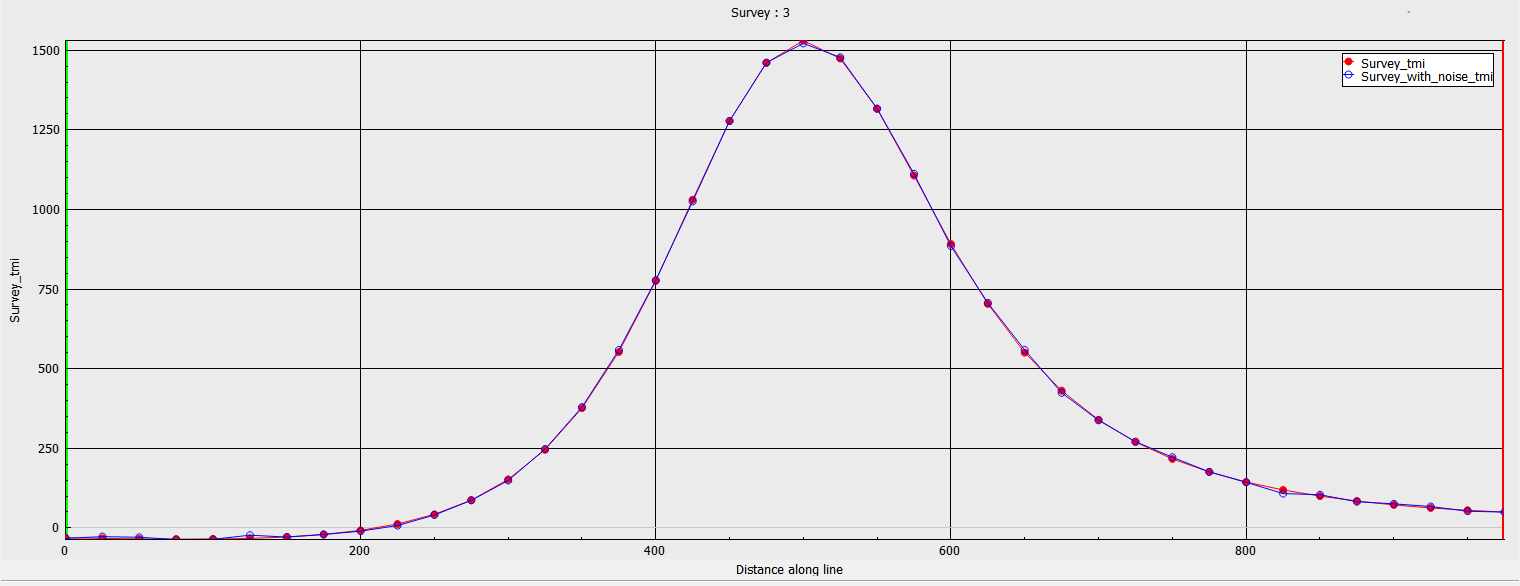
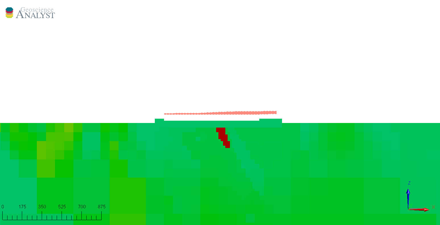
We are going to use the synthetic magnetic example shown below, and provided here. We added 20 nT of random Gaussian noise to the simulated data to emulate field conditions.

Constant floor

The simplest choice is to assign a constant value across the entire dataset - also referred to as “floor” uncertainties. It is related to the expected standard deviation of a Gaussian distribution if the noise is random.

In a real world context, the true noise level is unknown. It is common practice to estimate an appropriate floor by trial and error. The following three experiments demonstrate typical characteristics to be expected when attempting to determine an optimal noise floor.

Noise floor too high

With a high floor, the inversion is dominated by the regularization function and the data remains underfitted - there is coherent signal in the observed data that is not accounted for. The model is very smooth and we have a poor recovery of the shape of the susceptible body.

Noise floor too low

With this inversion, the uncertainties are intentionally set lower than the known random noise level. The inversion attempts to fit both the signal as well as the random noise. This gives rise to a spiky model with a lot of unwanted structure in the surface. The inversion also ran many more iterations in order to suppress the regularization function.

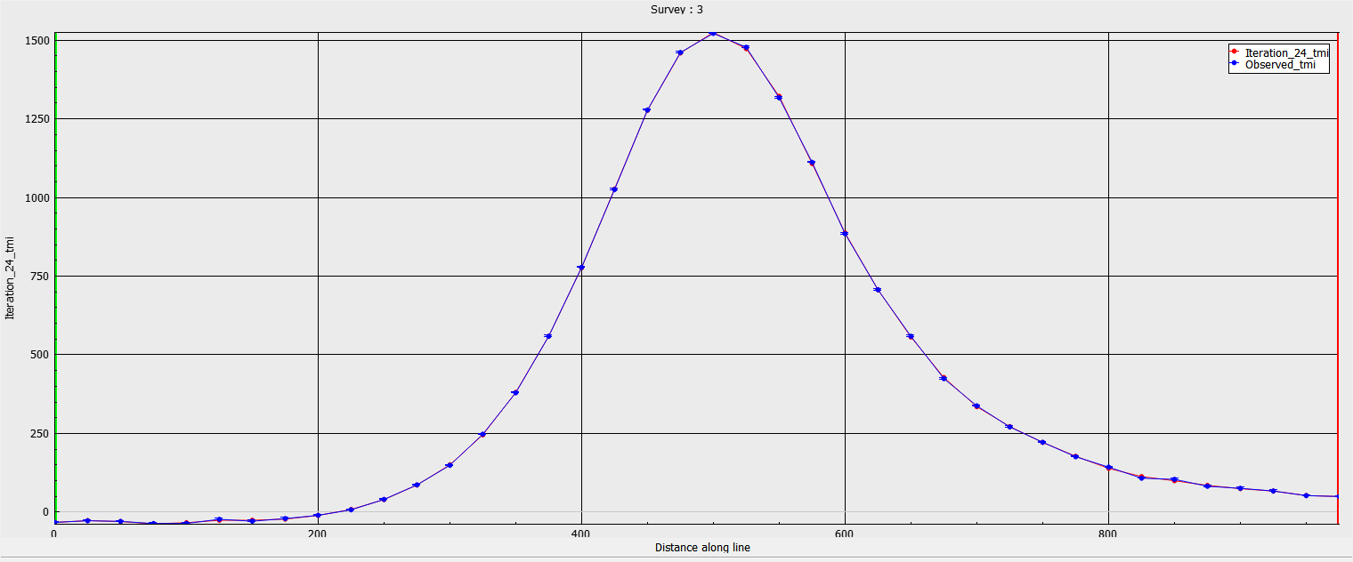
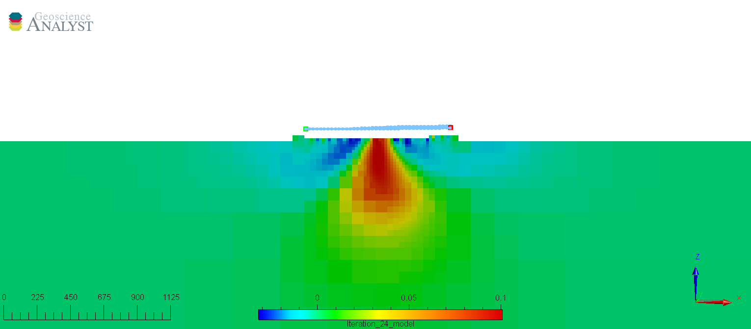
Optimal

The following inversion is with a well-chosen floor uncertainty. The model is fitting the data well without fitting the background noise. The model is smooth but retains the shape of the source.

Amplitude (%)

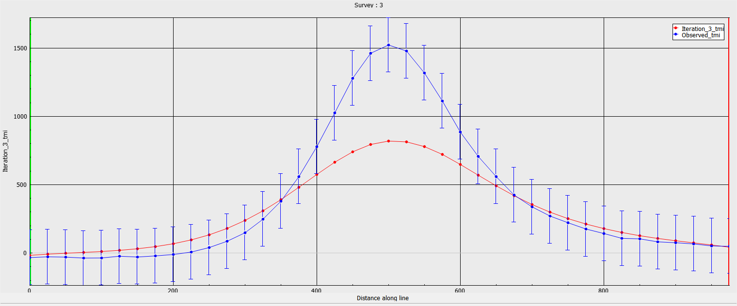
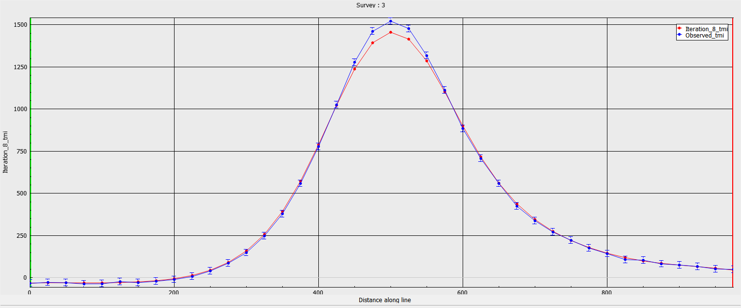
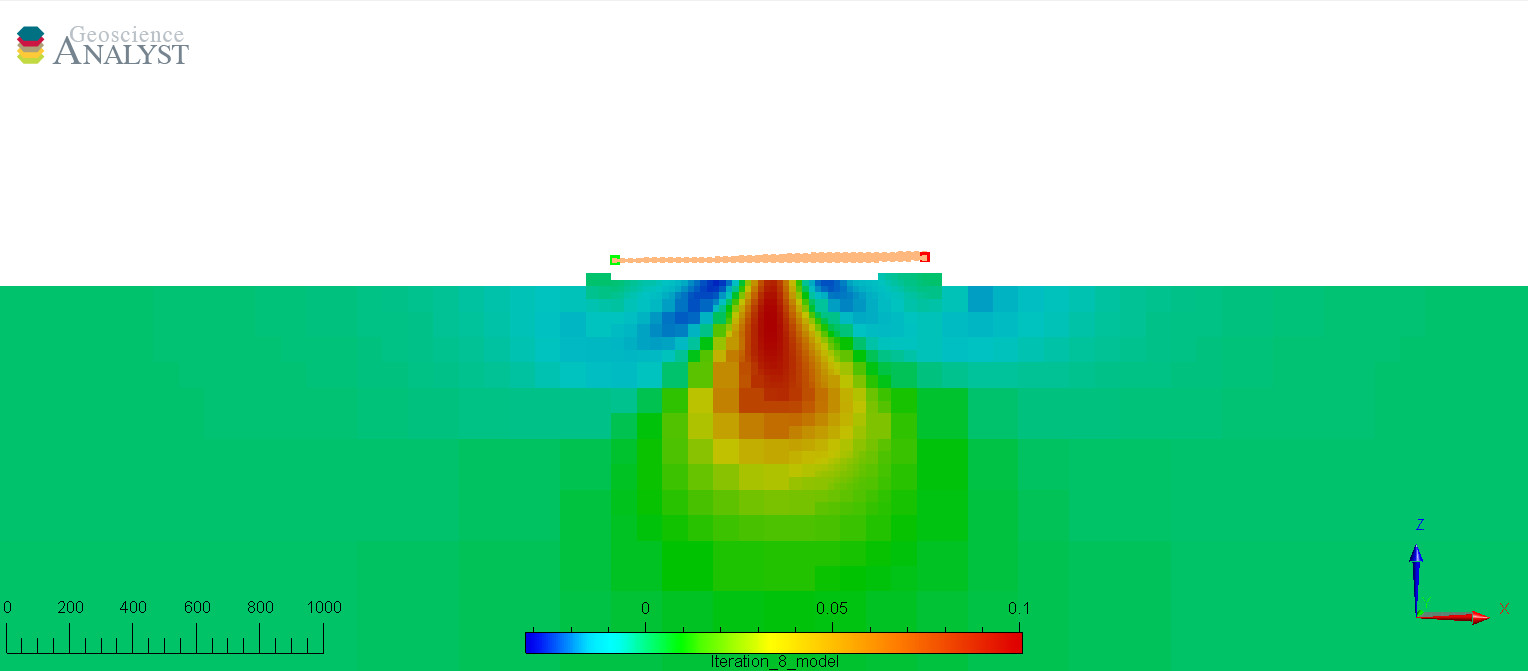
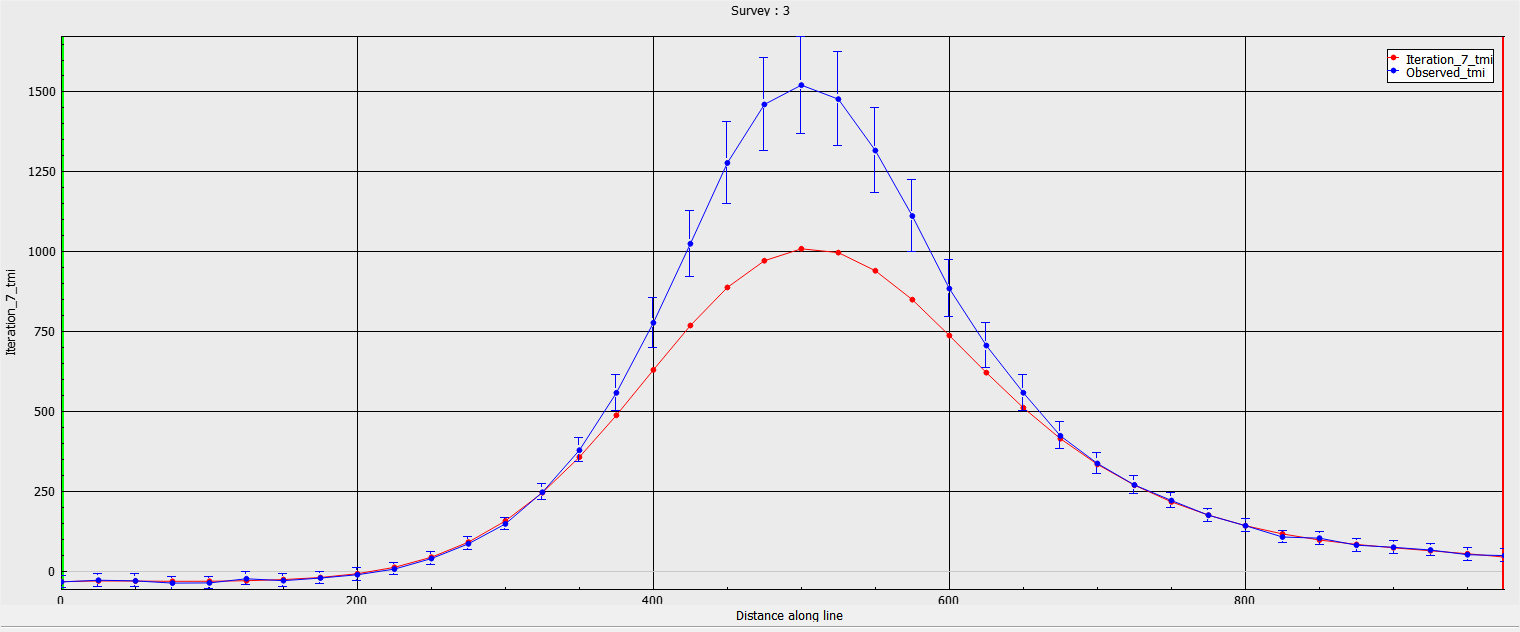
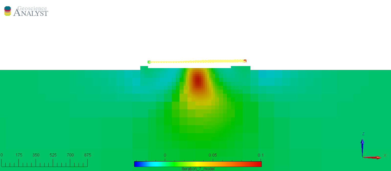
The second common strategy is to assign uncertainties based on the strength of the signal. In this scenario, we have assigned 10% of the amplitude of data plus a small floor (2 nT) to avoid singularity near zero:

\[ \mathbf{w} = \frac{1}{|\mathbf{d}^{obs}| + \epsilon} \]

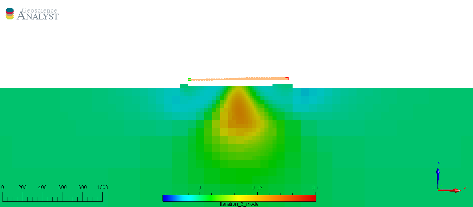
The figures below show the predicted data and recovered model after convergence of the inversion. We note that the predicted data fit well in the background, but underfit directly over the main anomaly. This is generally not desirable as the important portion of the geophysical signal is in the large amplitudes. The poor fit is reflected in the recovered low susceptiblity values and smooth shape of the magnetic body.

Summary

In this section we have demonstrated the effect uncertainties have on the outcome of an inversion, both on the data residuals and on the recovered model. It generally takes several inversions to determine appropriate uncertainties and involves some level of subjectivity from the user.