Background#
This section provides the mathematical background to understand the inversion algorithm. We are going to use standard terminology and nomenclature used in the literature as a framework. Even though we are going to use mathematical expressions, it is only a vehicle to help in understanding the influence of different parameters controlling the outcome of an inversion.
Forward simulation#
Before we start tackling the inverse problem, it is important to talk about the forward simulation. In other words, how does a computer generate geophysical data given a model and topography. We can generally write this in a simple form:
where
\(\mathbf{d}\) is the geophysical data (gravity, magnetic, voltages, etc.)
\(\mathbf{F}\) is some computer operation handling the physics
\(\mathbf{m}\) is a discrete model of physical property (density, susceptibility, conductivity, etc.)
Note that the forward simulation \(\mathbf{F}(\mathbf{m})\) varies in complexity depending on the type of geophysical survey: from a simple dense arrays for potential fields:
to elaborate partial differential equations for EM problems:
All that matters at this point is that SimPEG knows how to compute data given a model \(\mathbf{m}\).

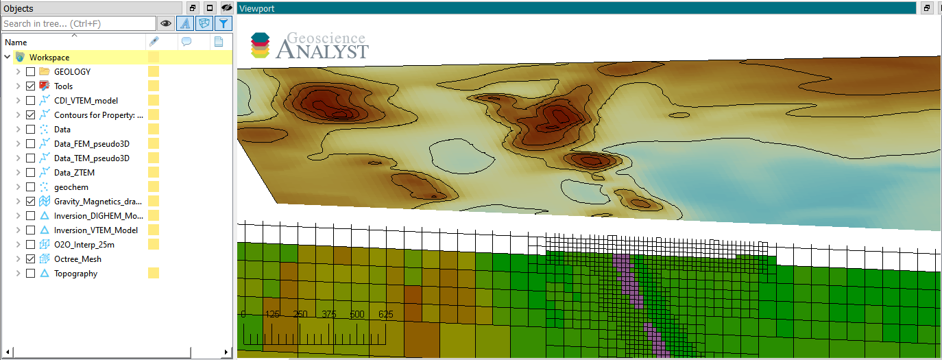
Figure showing simulated magnetic TMI data over the Flin Flon model (20 m resolution).
Example#
Let’s look at a simple 2 parameter problem to illustrate this concept:
The same expression can be written as linear operation of matrix \(\mathbf{F}\) multiplying a model \(\mathbf{m}\) such that
or
import numpy as np
from numpy.linalg import LinAlgError
F = np.c_[1, 2]
For given values for \(\mathbf{m}\), we have a way to compute data \(\mathbf{d}\). For example, for \(x = 0.5\) and \(y=0.25\)
np.dot(F, [0.5, 0.25])
array([1.])
Inverse problem#
In a mineral exploration context, we can collect data over the Earth but generally know little about the source of the signal (geology and physical properties). This is where the inversion process is required. In an ideal world we could simply perform the inverse of our forward simulation
but this operation is never possible in practice. First, there are too many unknowns compared to the amount of data, so \(\mathbf{F}^{-1}\) does not exist. Secondly, the data are generally noisy so that we would have:
This is referred to as an ill-posed problem. A common way to still find a (good) answer is to formulate inversion as a weighted least-squares optimization problem of the form:
such that we have a global function \(\phi(m)\) made up of two competing objectives:
\(\phi_d\) is the data misfit function that measures how well some model (\(\mathbf{m}\)) can fit the data
In linear form this can be written as
where the data weights \(\mathbf{W}_d\) are diagonal matrices with estimated data uncertainties. More details can be found in the data misfit module.
\(\phi_m\) is a regularization function measuring how well we fit geological assumptions
In linear form this can be written as
where the operator \(\mathbf{R}\) describe all functions used to guide the solution to a reference model \(\mathbf{m}_{ref}\). More details can be found in the regularization module. A solution for the minimum of the objective function can be computed by taking its partial derivatives with respect to the model and setting it to zero
The two functions are competing for what the model \(\mathbf{m}\) should look like - either fit the data (\(\phi_d\)) at all cost, or stay close to some geological assumptions (\(\phi_m\)). Finally we have our trade-off parameter \(\beta\), that determines the relative importance between these two competing objectives. More details about how the optimal \(\beta\) is determined can be found in the optimization section.
Example#
We can reuse the two-parameter problem above to illustrate the inverse problem. We are going to ignore the issue of noise for now and simply look at the under-determined problem $\( \large[\begin{array}{ccc} 1 & 2 \end{array}\large]\left[\begin{array}{ccc} x \\ y \end{array}\right] = 1\;. \)$
where we are giving data (\(d=1\)) and a linear operator \(\mathbf{F}=[1 \; 2]\).
Since \(\mathbf{F}\) does not have an inverse, we can instead solve the least-norm problem
which can be written as
Taking the derivative of \(\phi_d\) with respect to the model \(\mathbf{m}\) and setting it to zero yields
but even here \((\mathbf{F}^T \mathbf{F})^{-1}\) is singular and cannot be inverted directly as shown below
try:
    np.linalg.solve(np.dot(F.T, F), F.T * np.r_[1])
except LinAlgError as error:
    print(error)
Singular matrix
We can get around this by adding a small value to regularize the system such that
np.linalg.solve(np.dot(F.T, F) + 1e-12 * np.eye(2), F.T * np.r_[1])
array([[0.2],
       [0.4]])
We have found a solution to this under-determined problem: \(m = [0.2,\; 0.4]\). This result is known as the least-norm solution, which differs from the true answer \(m = [0.5, \;0.25]\). Other “better” solutions could be found if more information is provided to the inverse problem to push the model towards expected values. This will be the topic of the Regularization Section
