Mesh design#
An appropriately designed computational mesh is an important component to the geophysical inversion. There are both general and survey-specific strategies that may be used to design ‘good’ meshes for inversion. This section provides complementary details to the core Octree creation documentation, so readers may want to reference both.
Base parameters#
An Octree mesh can be though of as the combination of a base mesh and refinements. The base mesh is defined by the core extent, padding, and the base cell resolution. These concepts are explored in further detail in the following sub-sections.
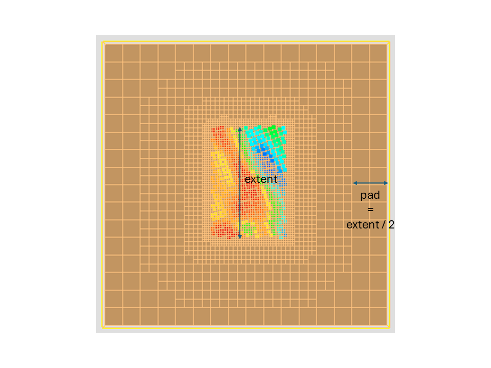
Mesh extent#
The mesh extent is provided as a geoh5py.object from which the bounding box is computed. For geophysical inversion this will in most cases be the geophysical survey object so that core region of the mesh will be centered below the data. For all geoh5py.BaseSurvey objects that contain a complement object (transmitters, base stations, current electrodes), the extent will be computed from the superposition of the object and it’s complement.
Base cell size#
Next, we need to define a base cell size for the core region. A few criteria need to be taken into consideration:
Sources/receivers separation
Terrain clearance (height above ground)
Modeling resolution (size of the target)
Numerical artefacts due to the discretization of topography decay sufficiently when receivers are roughly two cell dimensions away from the nearest edge or corner of a mesh cell in the air/earth boundary. For example, if the lowest drape height in given airborne survey is 60 m, a prudent cell size would be in the range of ~30 m. Another rule of thumb is that the cell size should be smaller than half the smallest data spacing. This is especially important for electrical methods where the electric field may be discontinuous and numerical artefacts may arise if the cells are not small enough to capture rapid changes in the field. For example, a 40m dipole direct-current survey would suggest a cell size around ~20m.
Padding cells#
As a general rule of thumb, the padding region should be at least as wide as the data extent in order to easily model features with wavelengths that may extend beyond the surveyed area.
In the case of EM modeling, we also need to consider the diffusion distance of the EM fields. The skin depth represents the distance over which the fields decay by a factor of \(1/e\). The skin depth can thus be used to add a padding distance that incorporates the minimum area within which the fields have any influence on the solution. The skin depth can be calculated for the frequency-domain system by:
where \(\rho\) is the expected resistivity of the background and \(f\) is the base frequency of the system.
Equivalently, for time-domain systems
where \(t\;(sec)\) is the largest time measured by the system, \(\rho \; (\Omega.m)\) is the expected resistivity of the background and \(\mu_0 \; (4 \pi * 1e-7)\) is the permeability of free space.
Refinements#
An octree mesh can be refined in specific regions - warranted for either numerical accuracy or modeling purposes. Fine cells can be “added” to the octree grid using various insertion methods that depend on the type of object used:
Radial: Add concentric spherical shells of cells around points. It is the default behaviour for
Points-like objects.Line: Add concentric tubes around line segments. It is the default discretization for line sources (EM loops) and
Curveobjects.Surface: Add layers of cells along triangulated surfaces in 3D. It is the default behaviour for
Surfaceobjects and mostly used to refine known boundaries between geological domain and topography.Horizon [Optional]: Add horizontal layers of cells below a triangulated surface computed from the input object’s vertices. This is a useful option to create a core region below the survey area.
See the Octree-Creation-App: Refinements section for more details.
For direct-current survey#
For EM methods, such as electrical direct-current surveys, the numerical accuracy of the forward simulation is the primary factor to decide on a mesh refinement strategy. It is important to have several small cells around each source and receivers for solving partial differential equations accurately. In this case, dipole source and receivers must be converted to a Points object in order to trigger a radial refinement. Concentric shells of cells are added around each source/receiver poles.
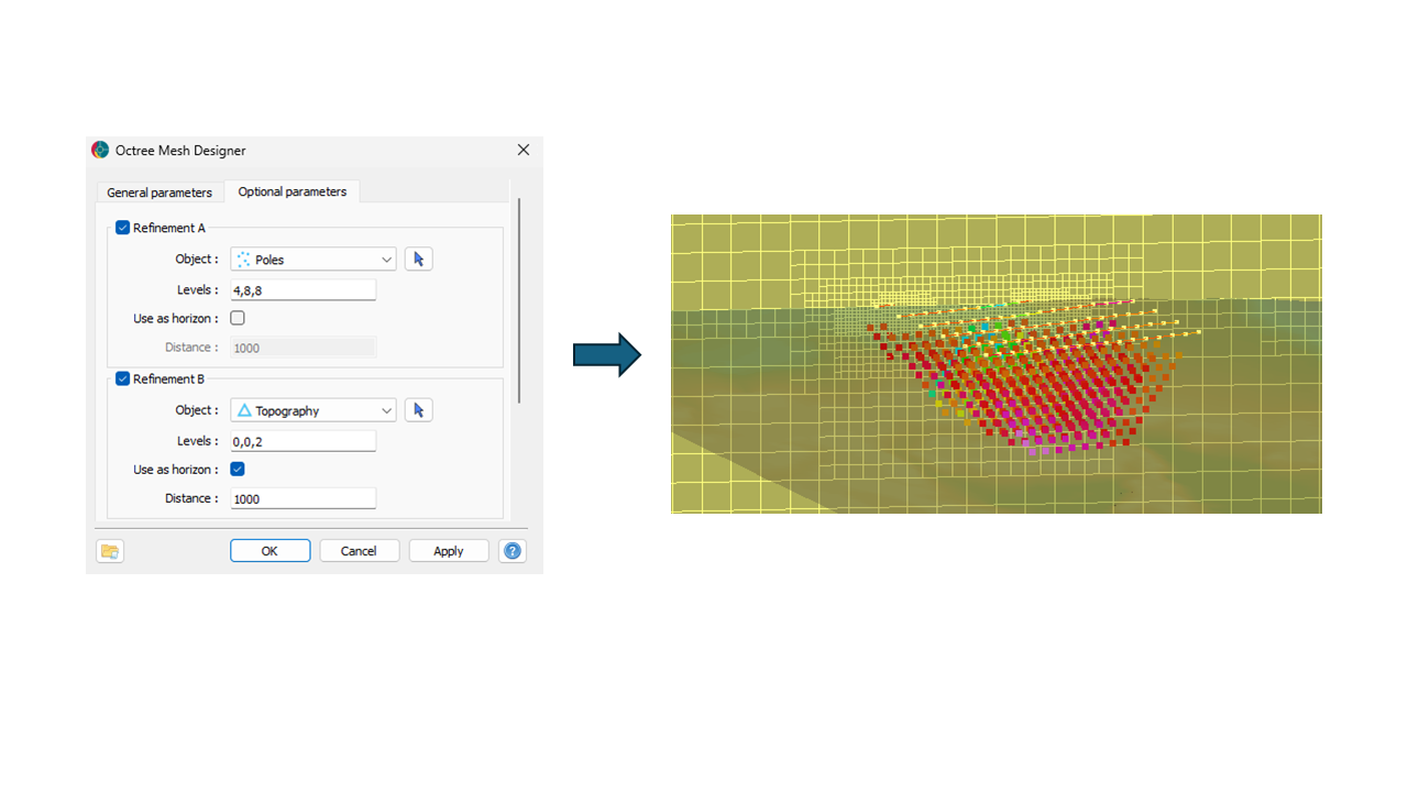
A second level of Surface refinement was added along the triangulated topography. Only coarse cells (3th octree level) were needed to preserve good continuity of the fields near the boundary of the domain.
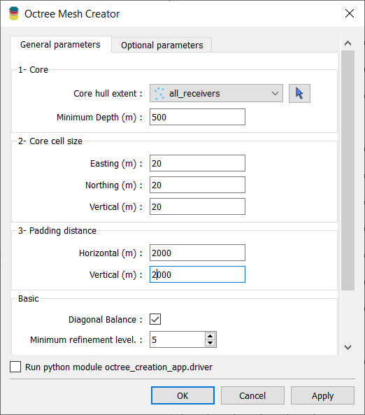
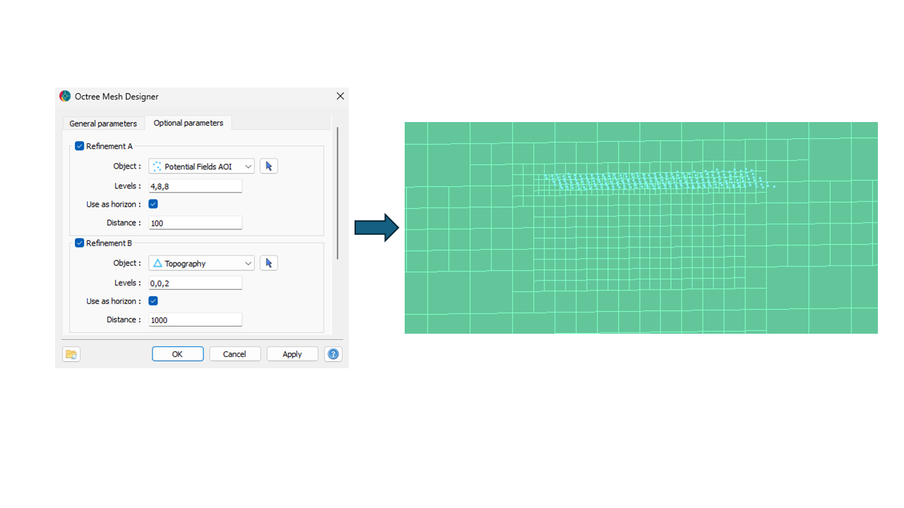
For gravity and magnetic surveys#
For potential field methods, the forward simulation is achieved via integration over prisms (linear operator) which is much less sensitive to the choice of discretization. Moreover, only cells below topography (active cells) are considered. For a more optimal mesh design, only fine cells are required at the air-ground interface. A horizon style refinement was used in order to add layers of fine cells below the footprint of the gravity and magnetic sensors. The maximum distance parameter was set to 100 m to reduce the number of small cells away from the receiver locations.
Auto-mesh#
The mesh can be generated in an automatic fashion where the meshing parameters are estimated from the geometry of survey and topography. The mesh parameter in the SimPEG ui.json files is optional. If the user leaves the mesh empty, a mesh will be created during setup for the subsequent inversion. This section describes how the meshing parameters are estimated for the auto-mesh routine.
Core parameters#
The auto-mesh routine refines radially about the survey locations and below the topography surface. The refinement for the survey creates three concentric shells of four cells at each level. The topography refinement places a single layer of two cells in the third octree level below the earth-air interface. The minimum level is set to six adding a base refinement to the whole mesh so that the cells in the padding region do not coarsen excessively.
Cell size#
The cell size will be chosen as half the median station spacing of the survey.
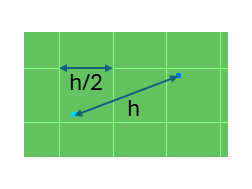
Padding#
The padding size can be estimated from the extent of the survey object. The auto-mesh will first compute the horizontal extent and take half of the largest extent (in x/y) for the horizontal padding parameters.