
Direct-current (DC) Resistivity Inversion#
This section focuses on the inversion of direct-current (DC) resistivity data generated from the Flin Flon resistivity model.
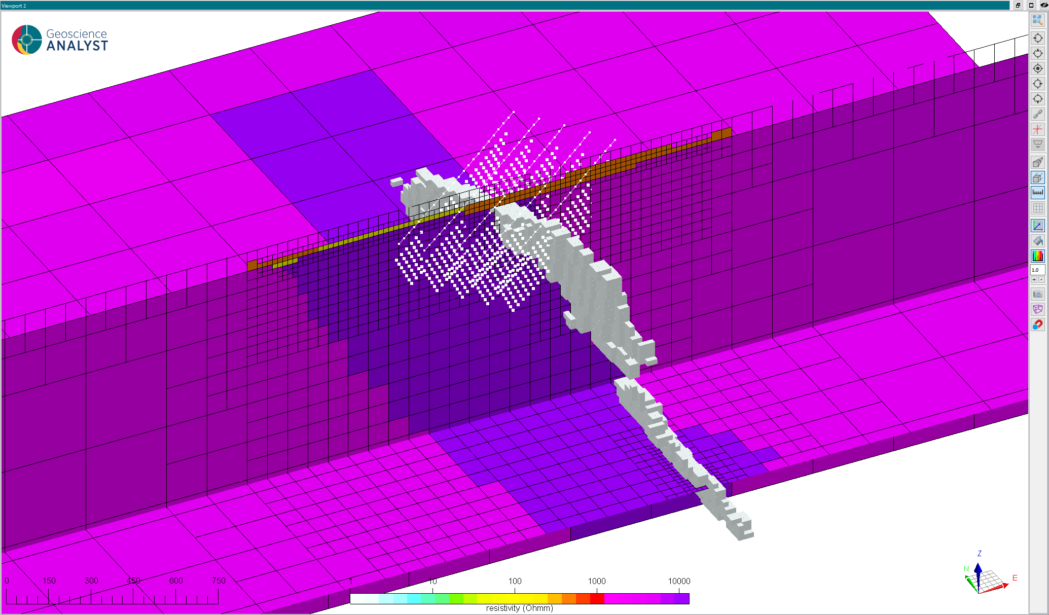
Fig. 19 Download here#
Data#
A ground dipole-dipole survey was simulated over the main ore body. The survey was acquired with 40 m dipole length, data measured on seven receivers per transmitter dipole. Line separation was set to 100 m (Figure 5).
The following parameters were used for the forward simulation:
Note the large contrast in apparent resistivity near surface between the western and eastern regions of the survey. This can be explained by a conductive alluvium layer West of the deposit. Lower apparent resistivities are also measured on the longer offsets over the ore body, hinting at a buried conductor.
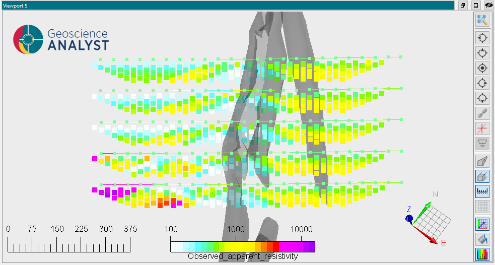
Fig. 20 Pseudo-sections of apparent resisitvity. Ore shell is shown in reference.#
Mesh creation#
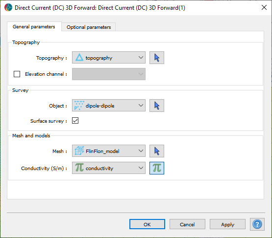
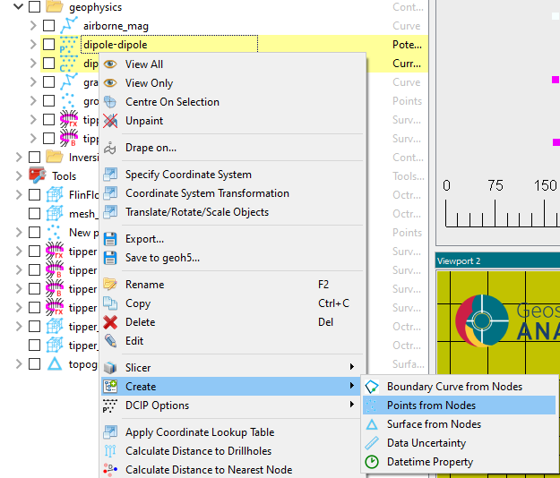
In preparation for the inversion, we create an octree mesh optimized for the DC resistivity survey. The survey is made of two objects: a Currents (sources) and a Potentials (receivers). In order to have good discretization around all pole locations, we first need to create an object that includes both components.
In the case of electric methods, the finest cell dimension should be at least half the dipole separation to guarantee that no two poles fall within the same mesh cell. This is important to assure good accuracy when computing voltage differences. We define our core param are as follow:
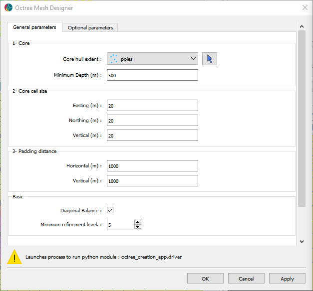
Fig. 21 Core mesh parameters.#
Refinements#
The first refinement adds more cells around each pole location, radially outward. This assures good numerical accuracy, espatially on the outer boundary of the survey area.
A second refinement is used along topography to get a coarse but continuous air-ground interface outside the area or interest.
The third refinement “horizon” is used to get a core region at depth with increasing cell size directly below the survey. This is our volume of interest most strongly influence by the data. We use a maximum distance of 100 m to limit the refinement away from the survey lines. In the case of remote electrodes, this parameter prevents from discretization finely everywhere in between.
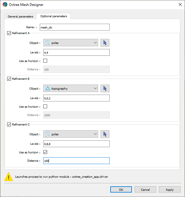
Fig. 22 Refinement strategy used for the direct-current modeling.#
See Mesh creation section for general details on the parameters.
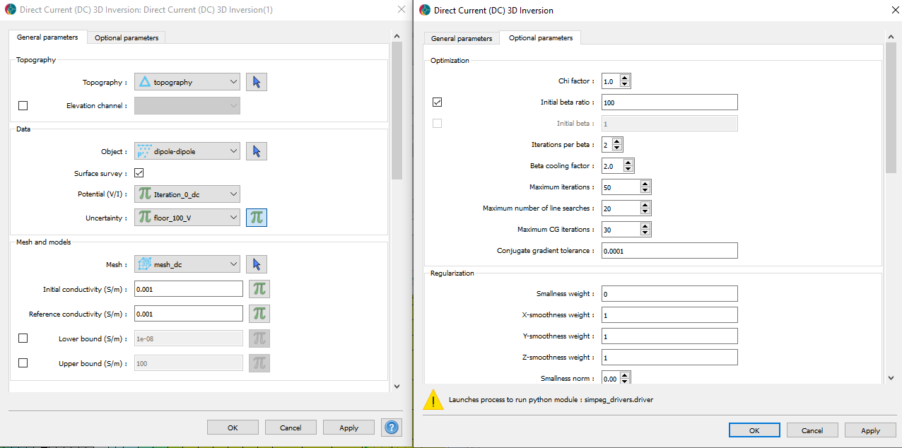
Unconstrained Inversion#
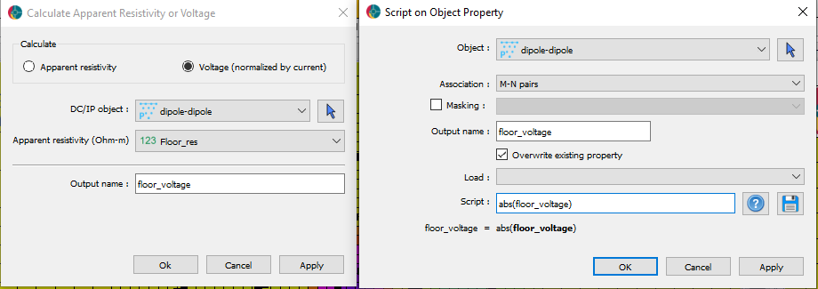
The direct-current data are inverted with uncertainties assigned based on a background resistivity value, then converted to potentials. This strategy is effective in scaling uncertainties relative to the dipole offsets.
1 - Create a constant resistivity value, set empirically in this case to 100 Ohm.m
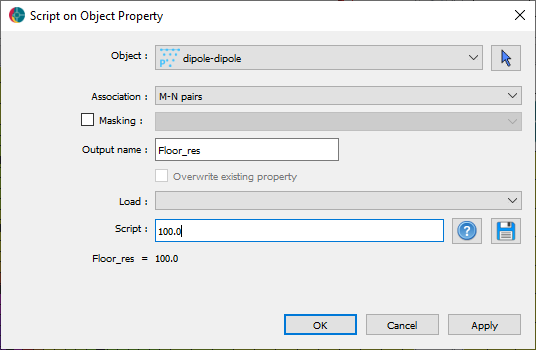
2- Convert the “floor resistivity” to voltages. The result needs to be absolute valued in order to be assigned as data uncertainties.
Having defined our uncertainties, we can proceed with the inversion.
The following figure shows the data fit and models recovered after convergence.
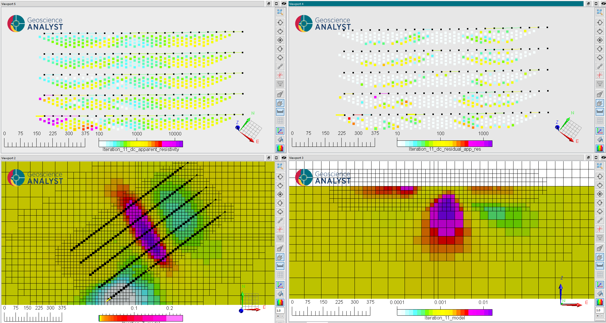
Fig. 23 (Top) (left) Predicted and (right) residuals data after reaching target misfit (iteration 11).#
(Bottom) Slices through the recovered conductivity model: (left) at 175 m elevation and (right) at 6072150 m N.
The data is generally explained well, although some correlated residuals are visible. This could warrant a second run with a slightly lower target Chi factor to push the data fit further.
On the modelling side, we note a large conductivity anomaly correlated with the ore body. The survey is able to define well the depth to top of the conductor but not the vertical extent. The inversion did identify the near-surface layers related to the conductive alluvium layer (West), which is slightly more conductive than the overburden layer (East).