
Joint Inversion#
This section introduces the methodology to invert multiple datasets jointly.
Joint Surveys Inversion#
As illustrated below, the joint surveys program allows to invert multiple datasets at once for a single physical property model. The goal is to combine complementary information from various geophysical surveys that sense the Earth differently.
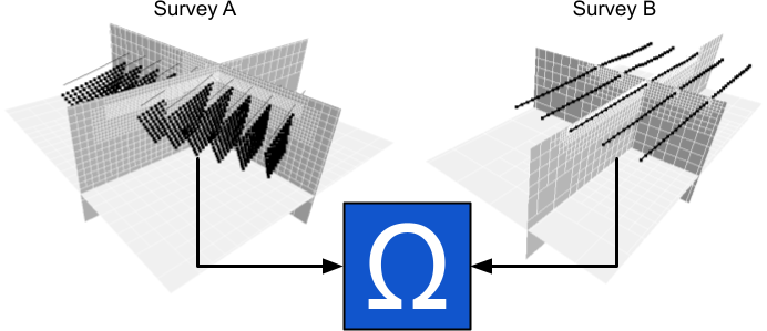
For example, a magnetotelluric survey is mostly sensitive to deep structures but can still be affected by local changes in resistivity near the sensor locations. A ground direct-current survey on the other hand is highly sensitive to near surface changes in resistivity. Inverting both surveys together would provide complementary information that improves our modeling capabilities overall.
This joint inversion problem does not require a coupling term - simply the summation of multiple misfit functions. Extending the objective function described in the inverse problem section, our new misfit function becomes
or
Since each misfit tries to update the same model values, the partial derivatives of each function is also a summation, such that
The joint survey inversion user requires a list of standalone inversion groups as input.
Joint Properties Inversion#
The more general joint inversion strategy tries to find commonality between different physical properties models. The goal is to invert for a common Earth model based on multiple geophysical surveys that might provide complementary information. For example, one could invert a direct-current resisitivity survey for the thickness of overburden, along with a gravity survey to highlight the density of targets under cover. Both geophysical survey are sensitive to different components of the sub-surface, but can greatly help each other in reducing ambiguity about the position and shape of physical property contrasts.
This kind of joint inversion requires a coupling term in order to tie those physical properties together.
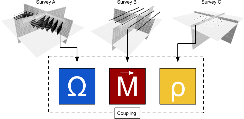
In this case, the model \(m\) is made up of N-number of sub-models, one per misfit function. The derivatives of the misfit function become
where the subscript \(j\) denotes the component of the model (either resistivity, magnetization or density). Each misfit function incluences a different subset of the model.
The following coupling terms are available through the SimPEG framework [HCK+17]:
Cross-gradient#
The cross-gradient regularization was first introduced by [GM03] to constrain electrical resistivity and seismic velocity inversions, but the same strategy applies to any physical property models. As the name states, the method employs the cross product on the spatial gradients of models such that
where \(\nabla \mathbf{m_A}\) and \(\nabla \mathbf{m_B}\) are the gradients for two distinct physical properties (density, magnetization components, resitivity, etc.). Since the cross-product of two vectors is also a vector, we use the total length (l2-norm) of the cross-product. The constraint is small (no impact) if the gradients of the models are either aligned or zero. Conversely, the measure becomes large if edges in the physical models are perpendicular with each other. Since we are attempting to minimize this function, this constraint will force model boundaries to occur at the same location or not at all.
It is possible to constrain more than two physical property models by adding multiple cross-gradient terms for every pair of models such that
and so on. Each term has a scaling parameter (\(\alpha\)) to control the importance of specific cross-gradient terms.
Linear Correspondence#
To be continued
Petrophysically Guided Inversion (PGI)#
To be continued
Mesh creation#
This section provides details on how to create the forward simulation meshes for each survey in preparation for a joint inversion. While all the misfit functions try to influence a model \(m\) defined on a global mesh, individual forward simulations \(\mathbb{F}^j(m)\) can be defined on sub-domains adapted to their specific array configurations. For example, an airborne EM simulation may require small cells in the air for numerical accuracy, while a dc-resisitivity survey only requires cells below ground at the transmitter-receiver pole locations.
To be continued