Constraints (Regularization)

This section focuses on the regularization functions, or constraints, that can be used to inject “geological knowledge” into the inversion process. More specifically, this section covers the weighted least-squares regularization functions:

• Conventional L2-norm

• General Lp-norms

While often referred to as an “unconstrained inversion”, one could argue that the conventional model norm regularizations do still incorporate some degree of geological information, at least in the form of physical property distribution. Exactly what kind of a priori information is available dictates the complexity of the constraints. For more advanced petrophysical and/or geometric constraints, see the Joint Inversion section.

L2-norm regularization

The conventional L2-norm regularization function imposes constraints based on the least-square measure with respect to the inversion model value

\[ \phi(m) = \| f(\mathbf{m}) \|_2^2 \;, \]

where \(f(\mathbf{m})\) is any linear function of the model \(\mathbf{m}\). The following sections introduce the conventional model “smallness” and “smoothness” functions.

Model smallness

In the seminal work of Tikhonov et al. [TASY95], the function \(f(\mathbf{m})\) simply measures the deviation between the inversion model from a reference

\[ f_s(\mathbf{m}) = \mathbf{m} - \mathbf{m}_{ref} \;, \]

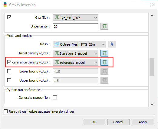
where \(\mathbf{m}_{ref}\) is a reference model. This function tries to keep the model “small”, as large deviations from the reference value are penalized more heavily. The reference model can vary in complexity, from a constant background value to a full 3D geological representation of the physical property. This constitutes our first constraint.

Model smoothness

A second set of terms can be added to the regularization function to apply constraints on the model gradients, or roughness of the solution. Following the notation used in Li. and Oldenburg [LiO98] and others before,

\[ f_x(\mathbf{m}) = \mathbf{G}_x (\mathbf{m} - \mathbf{m}_{ref}) \;, \]

where \(\mathbf{G}_x\) is a finite difference operator that measures the gradient of the model \(\mathbf{m}\) along one of the Cartesian directions (x for Easting). This function keeps the model “smooth”, as large gradients (sharp contrasts) are penalized strongly. Two additional terms are needed to measure the model gradients along the Northing (\(f_y\)) and vertical (\(f_z\)) direction.

Scaling

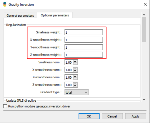
For 3D inverse problems, the full regularization function contains 4 terms: one for the reference model and three terms for the smoothness measures along the three Cartesian axes:

\[ \phi_m = \sum_{i = s,x,y,z} \alpha_i \| \mathbf{W}_i f_i(\mathbf{m}) \|_2^2 \]

Note that we have added scaling parameters \(\alpha_i\) to each function. The role of those multipliers is two-fold:

• User-defined weights to emphasize the contribution of a particular function

• Dimensionality scaling to level the functions with each other.

Dimensionality scales arise from the difference operators:

\[ \phi_x(m) = \sum_{i=1}^{N_{fx}} \left(\frac{\Delta m_i}{h_{xi}}\right)^2 \]

such that \(\Delta m_i\) is the difference in model values between two cells separated by a distance \(h_{xi}\) along the x-axis. When adding together the [reference](#Model smallness) and [model smoothnedd](#Model smoothness) terms in the regularization, it is obvious that the scale factor of \(h^{-2}\) would favor \(\phi_m\) to have a larger impact on the solution. The standard practice is to weight down the influence of the reference model accordingly.

Note

For all SimPEG inversions, dimensionality scaling of \(h^2\) is applied directly for the gradient terms by the program, allowing the default state to be all 1s for simplicity.

Model weights (future option)

Any of the regularization functions mentioned above can be further augmented with weights associated with each model cell such that

\[ \phi_i = \| \mathbf{W}_i f_i(\mathbf{m}) \|_2^2 \]

where \(\mathbf{W}_i\) contains positive values that change the relative strength of the regularization function in specific volumes of the 3D space. This is typically done for advanced constraints to reflect variable degrees of confidence in the reference geological model (e.g. high near the surface, low at depth). This option is currently not available but it is planned to be included in geoapps v0.12.0.

Sparse regularization

It is possible to generalize the conventional least-squares approach such that we can recover different solutions with variable degrees of sparsity Fournier and Oldenburg [FO19]. The goal is to explore the model space by changing our assumption about the character of the solution, in terms of volume of the anomalies and sharpness of contrasts between domains. We can do this by changing the “ruler” by which we evaluate the model function \(f(\mathbf{m})\).

Approximated \(L_p\)-norm

Since the general \(L_p\) norm is not linear with respect to the model, an approximation is used where

\[ \phi(m) = \| f(\mathbf{m}) \|_p \]

\[ \sum_{j}^M {|f(m)_i |}^p \approx \sum_{i} {\frac{ {f(m)_i}^2}{\left( {{f(m)_i}}^{2} + \epsilon^2 \right)^{1-p/2 }}} \]

where \(p\) is any constant between \([0,\;2]\). This is a decent approximation of the \(l_p\)-norm for any of the functions presented in the L2-norm section.

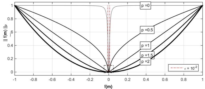
Note that choosing a different \(l_p\)-norm greatly changes how we measure the function \(f(m)\). Rather than simply increasing exponentially with the size of \(f(m)\), small norms increase the penalty on low \(f(m)\) values. As \(p\rightarrow 0\), we attempt to recover as few non-zero elements, which in turn favour sparse solutions.

Since it is a non-linear function with respect to \(\mathbf{m}\), we must first linearize it as

\[ \| f(\mathbf{m})_i \|_p \approx \| \mathbf{R}_i f(\mathbf{m})_i\| \]

where

\[ \mathbf{R}_i = {\frac{1}{\left( {{f(m)^{(k-1)}_i}}^{2} + \epsilon^2 \right)^{1-p/2 }}}\,. \]

Here the superscript \((k)\) denotes the inversion iteration number. This is also known as an iterative re-weighted least-squares (IRLS) method. For more details on the implementation refer to Fournier and Oldenburg [FO19].

The next two sub-sections apply this methodology to the model smallness and model smoothness regularizers.

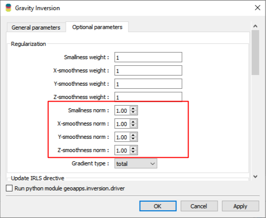
Smallness norm model

The first option is to impose sparsity assumptions on the model values.

\[ \phi(m) = \| (\mathbf{m} - \mathbf{m}_{ref} \|_p \;. \]

That is, we ask the inversion to recover anomalies that have small volumes but large physical property contrasts. This is desirable if we know the geological bodies to be discrete and compact (e.g. kimberlite pip, dyke, etc.). The example below demonstrates the outcome of an inversion for different combinations of norms applied to the model

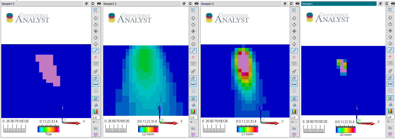
The figure above shows vertical sections through the true and recovered models (from left to right) with L2, L1 and L0-norm on the model values.

Note that as \(p \rightarrow 0\) the volume of the anomaly shrinks to a few non-zero elements while the physical property contrasts increase. They generally agree on the center position of the anomaly but differ greatly on the extent and shape.

No smoothness constraints were used (\(\alpha_{x,y,z} = 0\)), only a penalty on the reference model (\(m_{ref} = 0\)).

All those models fit the data to the target data misfit and are therefore valid solutions to the inversion.

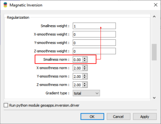
Smoothness norm model

Next, we explore the effect of applying sparse norms on the model gradients. We have two options.

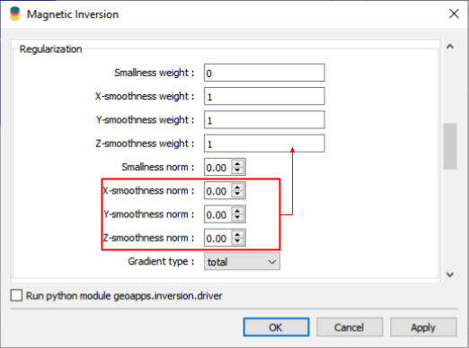
Gradient type: Total

The favoured approach is to measure the total gradient of the model

\[ \phi(m) = \| |\nabla \mathbf{m}| \|_p \]

or in matrix form

\[ \phi(m) = \| \sqrt{(\mathbf{G}_x \mathbf{m})^2 + (\mathbf{G}_y \mathbf{m})^2 + (\mathbf{G}_z \mathbf{m})^2} \|_p \;. \]

In this case, we are requesting a model that has either large or no (zero) gradients. This promotes anomalies with sharp contrast and constant values within.

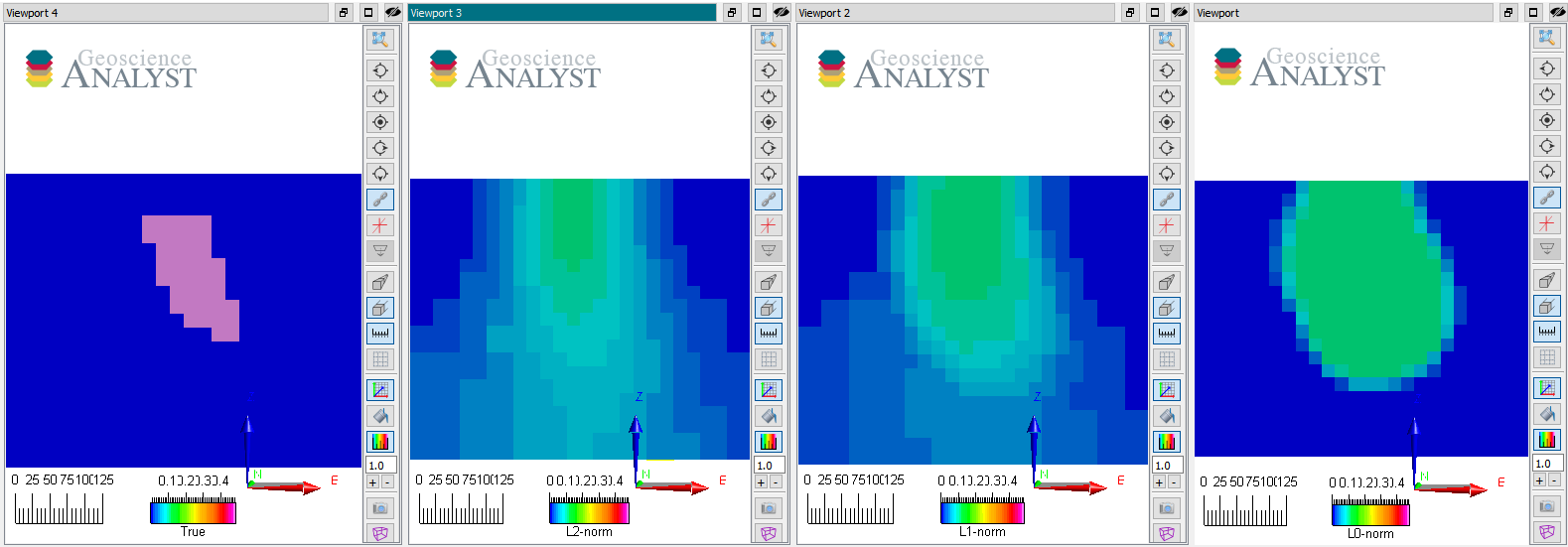
The figure above shows vertical sections through the true and recovered models (from left to right) with L2, L1 and L0-norm on the model gradients.

No reference model was used (\(\alpha_s = 0\)) with uniform norm values on all three Cartesian components.

All those models also fit the data to the target data misfit and are therefore valid solutions to the inversion. Note that as \(p \rightarrow 0\) the edges of the anomaly become tighter while variability inside the body diminishes. They generally agree on the center position of the anomaly but differ greatly on the extent and shape.

Note

In the literature, the majority of studies on sparse norms use the L1-norm on the model gradients, also called Total Variation inversion. While the implementation may differ slightly, the general \(l_p\)-norm methodology presented above covers this specific case. We can re-write

\[ \sum_{i} {|f(m)_i |}^p \approx \sum_{i} {\frac{ (\mathbf{G}_x \mathbf{m})_i^2 + (\mathbf{G}_y \mathbf{m})_i^2 + (\mathbf{G}_z \mathbf{m})_i^2}{\left( (\mathbf{G}_x \mathbf{m})_i^2 + (\mathbf{G}_y \mathbf{m})_i^2 + (\mathbf{G}_z \mathbf{m})_i^2 + \epsilon^2 \right)^{1-p/2 }}} \;. \]

Then for \(p=1\)

\[ \phi(m) \approx \sum_{i} \sqrt{(\mathbf{G}_x \mathbf{m})_i^2 + (\mathbf{G}_y \mathbf{m})_i^2 + (\mathbf{G}_z \mathbf{m})_i^2} \;, \]

we recover the total-variation (TV) function. Lastly for \(p=2\)

\[ \phi(m) = \sum_{i} (\mathbf{G}_x \mathbf{m})_i^2 + (\mathbf{G}_y \mathbf{m})_i^2 + (\mathbf{G}_z \mathbf{m})_i^2 \]

we recover the smooth regularization.

Gradient type: Components

Alternatively, we can treat each gradient term independently such that

\[ \phi(m) = \| \mathbf{G}_x \mathbf{m} \|_p + \| \mathbf{G}_y \mathbf{m} \|_p + \| \mathbf{G}_z \mathbf{m} \|_p \]

This formulation tends to recover box-like anomalies with edges aligned with the Cartesian axes. This is generally not desirable unless the gradients can be rotated in 3D.

Mixed norms

The next logical step is to mix different norms on both the smallness and smoothness constraints. This gives rise to a “space” of models bounded by all possible combinations on \([0, 2]\) applied to each function independently.

To be continued…