Joint Cross Gradient Inversion

The joint cross-gradient inversion strategy allows to find commonality between multiple physical property models by minimizing the cross-product of their spatial gradients. This method is particularly useful when inverting for different physical properties that are expected to have similar spatial structure.

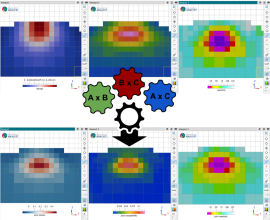
Fig. 12 Recovered models from (left to right) a gravity, magnetic and resistivity survey; (top) without constraints and (bottom) with a cross-gradient constraint to encourage common structure across all models.

For example, a geological features may be responsible for a magnetic, gravity and electrical anomaly. Even though the three datasets may have different sensitivities to subsurface features, it would be ideal if their respective magnetic, density and resistivity models shared some resemblance. Within a purely unconstrained inversion framework however, this is rarely the case.

By minimizing the cross-gradient of the two models, we can encourage the inversion to find a common structure across all models, and therefore provide complementary information about the subsurface structure. By combining this information, we can significantly reduce inversion ambiguity and obtain a more accurate and robust model of the subsurface.

Background

The cross-gradient regularization was first introduced by [GM03] to constrain electrical resistivity and seismic velocity inversions, but the same strategy applies to any physical property models. As the name states, the method employs the cross product on the spatial gradients of models such that

\[\phi_c(\mathbf{m_A},\mathbf{m_B}) = \sum_{i=1}^{M} \| \nabla \mathbf{m_A}_i \times \nabla \mathbf{m_B}_i \|^2\]

where \(\nabla \mathbf{m_A}\) and \(\nabla \mathbf{m_B}\) are the gradients for two distinct physical properties (density, magnetization components, resitivity, etc.). Since the cross-product of two vectors is also a vector, we use the total length (l2-norm) of the cross-product. The constraint is small (no impact) if the gradients of the models are either aligned or zero. Conversely, the measure becomes large if edges in the physical models are perpendicular with each other. Since we are attempting to minimize this function, this constraint will force model boundaries to occur at the same location or not at all.

The full regularization function for the joint cross-gradient inversion, with conventional Tikhonov regularization for each model, becomes

\[\phi_m = \sum_{i=s,x,y,z} \alpha_i^A \| \mathbf{W}_i^A \mathbf{m_A} \|^2 + \sum_{i=s,x,y,z} \alpha_i^B \| \mathbf{W}_i^B \mathbf{m_B} \|^2 + \alpha_c \phi_c(\mathbf{m_A},\mathbf{m_B})\]

made up of nine terms in total: four for each model and one cross-gradient term.

It is possible to constrain more than two physical property models by adding multiple cross-gradient terms for every pair of models such that

\[\phi_c(\mathbf{m_A},\mathbf{m_B}, \mathbf{m_C}) = \alpha_{AB} \phi(\mathbf{m_A},\mathbf{m_B}) + \alpha_{AC}\phi(\mathbf{m_A},\mathbf{m_C}) + \alpha_{BC} \phi(\mathbf{m_B},\mathbf{m_C})\]

and so on. Each term has a scaling parameter (\(\alpha\)) to control the importance of specific cross-gradient terms. Further automated rescaling is available, as explained in the Iterative re-scaling section.

Interface

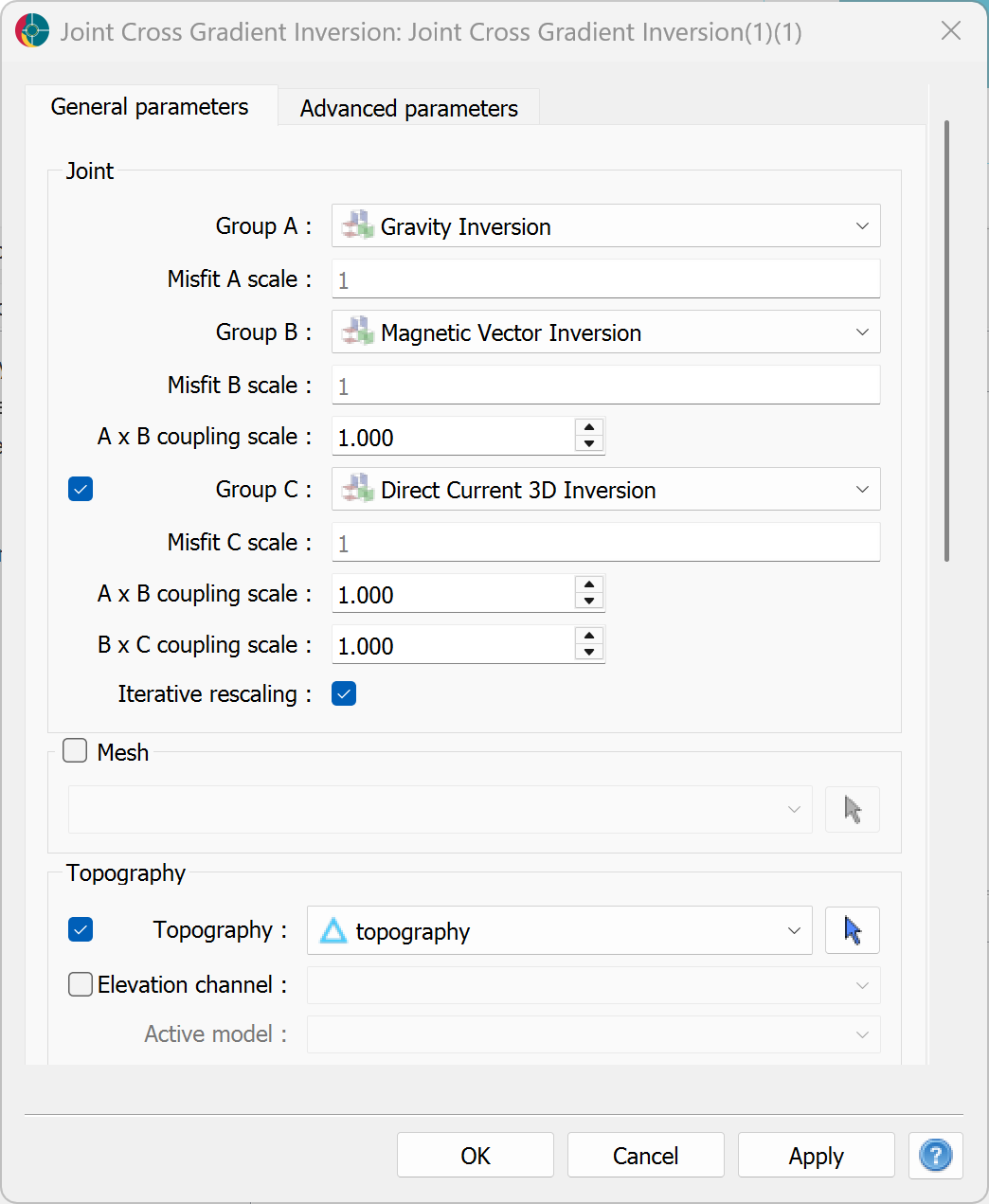
The joint cross-gradient inversion user requires the following input parameters:

Input parameters

• Group A, B and C:

  : Standalone inversion groups to be included in the joint inversion. Up to three groups can be included in the joint inversion, but only two are required. Each group should be fully defined and runnable as a standalone inversion problem, with its own survey and mesh.

• Misfit scale A, B and C:

  : For each standalone inversion group, a scaling factor to be applied to the misfit function. This allows to scale the uncertainties of individual surveys.

• Coupling scales AxB, AxC and BxC:

  : For each pair of models, a scaling factor to be applied to the cross-gradient function. This allows to control the importance of specific cross-gradient terms. The higher the value, the more the inversion will try to align the edges of the models. Setting the value to zero will effectively turn off the coupling between the two models

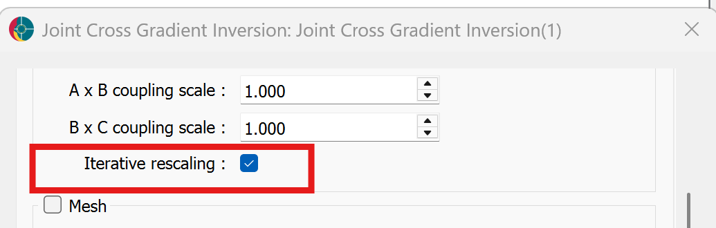
• Iterative rescaling:

  : Optional iterative rescaling of the coupling terms relative to other components of the regularization function. More details provided in the Iterative re-scaling section.

Inversion mesh

Optional octree mesh object used for by regularization and storing the models. If not supplied, a new mesh is generated by combining the finest cell size encountered across all standalone meshes. See details in the inversion mesh section.

Advanced parameters

By default, the regularization parameters of the standalone inversions are used, allowing for maximum flexibility in controlling the character of individual models. Otherwise, when the Regularization group is activated, global parameters can be used across all the sub-regularization functions for more consistent behavior.

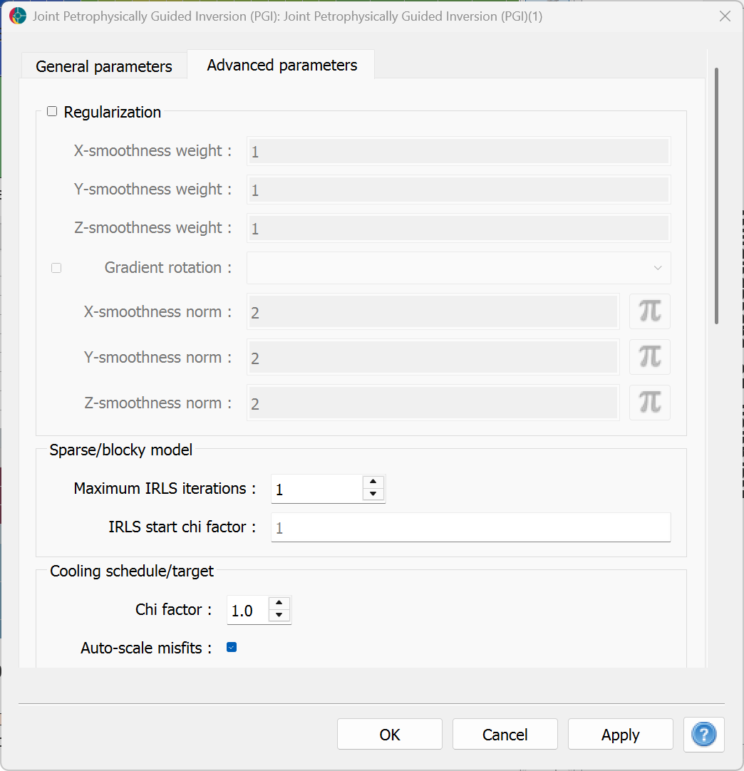
All other parameters related to the optimization of the standalone inversions are overridden by the joint inversion framework.

• Auto-scaling of misfit functions:

  By default, an auto-scaling of the misfit functions is applied at each iteration, such that the contribution of each survey to the model update is balanced. This is particularly important when the surveys have different units or sensitivities. More details about the auto-scaling strategy can be found in the Auto-scaling of misfit functions section.

Iterative re-scaling

As previously discussed in the Dimensionality Scaling section, the different components of the regularization function can have different units. This can lead to an unbalanced inversion process, where the model is updated mostly based on one component of the regularization function, while the others have little influence. This is particularly true for the cross-gradient term.

To address this issue, an Iterative rescaling option allows to automatically re-scale the coupling terms relative to the other components in an automated way at each iteration.

To define a scaling strategy, we can compare the dimensions of the derivatives of the smallness (reference model) term

\[\; dim\; \frac{\delta \phi_s}{\delta m} = [m] \;,\]

to the dimensions of the derivative of the cross-gradient term

\[\; dim\; \frac{\delta \phi_c}{\delta m} = \frac{[m]^3}{[h]^4} \;.\]

The two derivatives have different dimensions by a factor of \([m]^2/[h]^4\). We therefore define an iterative scaling factor for the cross-gradient term as

\[\;\alpha_c^{(k)} = \alpha_c \left[\frac{m^{(k)}_{max} - m^{(k)}_{min}}{h^2}\right]^{-2} \]

where \(m^{(k)}_{max}\) and \(m^{(k)}_{min}\) are the maximum and minimum model values at iteration \(k\), and \(h\) is the smallest cell size of the mesh. This scaling factor brings the derivatives of the cross-gradient terms to be dimensionally equivalent to the derivatives of the other terms in the regularization function.