Joint Surveys Inversion

The joint surveys inversion framework allows to invert multiple datasets at once for a single physical property model. The goal is to combine complementary information from various geophysical surveys that sense the Earth differently.

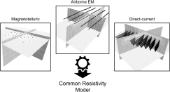
For example, a magnetotelluric survey is mostly sensitive to deep structures but can still be affected by local changes in resistivity near the sensor locations. A ground direct-current survey on the other hand is highly sensitive to near surface changes in resistivity. Inverting both surveys together would provide complementary information that improves our modeling capabilities overall.

Background

The joint survey inversion does not require a coupling term - simply the summation of multiple misfit functions influencing the same model. The global misfit function becomes

\[\phi_d = \phi_d^A + \phi_d^B + ...\]

or

\[\phi_d = \sum_{j=A, B, C} \phi_d^j\]

Since each misfit tries to update the same model values, the partial derivatives of each function is also a summation, such that

\[\frac{\delta \phi_d}{\delta m} = \sum_{j=A, B, C} \frac{\delta \phi_d^j}{\delta m}\]

Interface

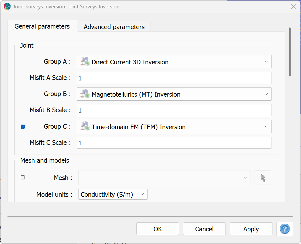
The joint survey inversion user requires a list of standalone inversion groups as input.

Input parameters

• Group A, B and C

  : Standalone inversion groups to be included in the joint inversion. Up to three groups can be included in the joint inversion, but only two are required. Each group should be fully defined and runnable as a standalone inversion problem, with its own survey and mesh. Any other regularization or optimization parameters will be ignored and overridden by the joint inversion framework.

• Misfit Scales A, B and C

  : For each standalone inversion group, a scaling factor to be applied to the misfit function. This allows to scale the uncertainties of individual surveys.

Inversion mesh

Optional octree mesh object used for by regularization and storing the models. If not supplied, a new mesh is generated by combining the finest cell size encountered across all standalone meshes. See details in the inversion mesh section.

Advanced parameters

All advanced parameters related to the regularization and optimization of the standalone inversions are ignored and overridden by the joint inversion framework.

Auto-scaling of misfit functions

By default, an auto-scaling of the misfit functions is applied at each iteration, such that the contribution of each survey to the model update is balanced.

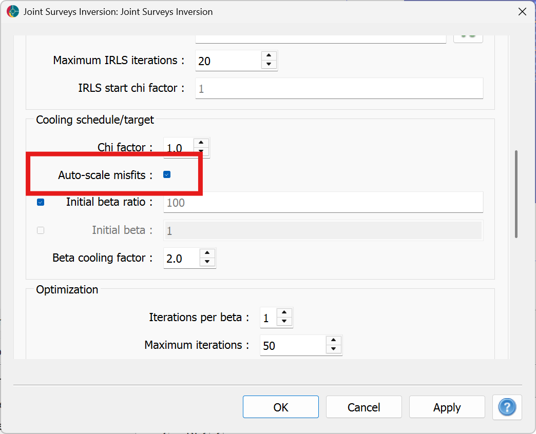
This is particularly important when the surveys have different units or sensitivities. This auto-scaling strategy prevents the inversion from being dominated by a single survey, or overfitting a survey while the others are still far from their target.

The scaling factor for each survey is computed as the ratio between the achieved chi factor to the maximum chi factor of all surveys, scaled by the cooling factor of the trade-off parameter, such that

\[\text{scale}_j = 1 - (1 - \Delta\beta) \frac{\chi_{max} - \chi_j}{\chi_{max}}\]

where \(\Delta \beta\) is the chosen cooling factor of the trade-off parameter, and \(\chi_j\) are the chi factors for each survey. Chi factors are computed as the ratio between the data misfit and the number of data points:

\[\chi_j = \frac{\phi_d^j}{N_j} \,.\]

The misfit with the highest chi factor will have a scaling factor of 1, while the other misfits will have a scaling factor between \(\delta \beta\) and 1, depending on how far their chi factor is from the maximum. In other words, misfits with the lowest chi factors are scaled down by the same amount as the trade-off parameter, effectively cancelling the cooling step as long as their chi factor remains small. As the inversion progresses and the chi factors of all surveys reach a similar value, the scaling factors will increase towards 1, allowing all misfits to progress towards their target.